Classical complexity reductions among hard lattice problems

Table of Contents

SVP and CVP Problem Instances
- The Closest Vector Problem
  - Exact Closest Vector Problem (CVP)
  - Approximate Closest Vector Problem ( $𝛾$ -CVP)
Reductions among exact problems

The difficulty of solving a hard lattice problem depends significantly on the choice of its parameters. One cannot meaningfully discuss cryptographic constructions — especially FHE schemes — without first understanding the complexity landscape of lattice problems. This post describes several classical (i.e., non-quantum) reductions among different lattice problems. If you only care about the results, here’s a visual representation of the complexity of solving these problems as a function of approximation ratio $𝛾$ :

Hardness of approximating SVP and CVP as function of approximation parameter gamma

This chart is taken from ¹ with the following change: Khot’s seminal GapSVP $𝛾$ inapproximability result ², where $𝛾 (𝑛) \leq 2 (l o g 𝑛) 1 / 2 - 𝜖$ was proved to be inapproximable, has been updated with Haviv-Regev’s inapproximability result from ³ where $𝛾 (𝑛) \leq 𝑛 𝑐 / l o g l o g 𝑛$ .

SVP and CVP Problem Instances

Recall that an NP Optimization (NPO) problem is a minimization or maximization problem where the goal is to find an optimal solution from a set of possible solutions. An approximation algorithm for an NPO problem always returns a valid solution, but with the caveat that it may not be optimal. However, even in the worst case, these algorithms do provide the guarantee that the output will be no worse than $𝛾 \in ℝ (𝛾 \geq 1)$ times the optimal. $𝛾$ is called the approximation ratio and its value depends on the algorithm, not the problem instance.

Both SVP and CVP are NP Optimization (NPO) problems. Recall that an SVP $𝛾$ problem instance consists of a lattice $L$ specified by a basis $𝐁 \in ℝ 𝑛 \times 𝑛$ and an approximation ratio $𝛾$ . The goal is to find a short (non-zero) lattice vector $⃗ 𝑥 \in L (𝐁)$ such that $⃗ 𝑥$ is at most $𝛾$ times longer than the shortest (non-zero) vector in $L (𝐁)$ . In case of CVP $𝛾$ , in addition to $𝐁$ and $𝛾$ , we are also given a target vector $⃗ 𝑡 \in ℝ 𝑛$ , and the goal is to find some lattice vector $⃗ 𝑦 \in L$ that is at most $𝛾$ times longer than the shortest possible distance between $⃗ 𝑡$ and any point in $L$ .

The three different flavors of exact SVP — Search-SVP, Opt-SVP, and Decisional-SVP — as well their approximate versions — Approx-SVP $𝛾$ and GapSVP $𝛾$ — were described in detail in the previous post. The next subsection formally defines the exact and approximate versions of Closest Vector Problem (CVP). Readers already familiar with CVP can safely skip the next subsection.

The Closest Vector Problem

The distance between any lattice vector $⃗ 𝑥 \in L$ and a point $⃗ 𝑡 \in ℝ 𝑛$ in space is defined as the usual Euclidean distance (or any $ℓ 𝑝$ norm) between two points in space: $Δ (⃗ 𝑡, ⃗ 𝑥) : = ‖ ⃗ 𝑡 - ⃗ 𝑥 ‖$ . However, a lattice is an infinite collection of points, so defining the distance between a point and the entire lattice requires a new definition:

(Distance from a Lattice, Closest Vector)

Let $L$ be a full-rank lattice specified by a basis $𝐁 \in ℝ 𝑛 \times 𝑛$ , and let $⃗ 𝑡 \in ℝ 𝑛$ be an arbitrary point in space. Then, the distance between $⃗ 𝑡$ and $L$ is defined as the minimum distance between $⃗ 𝑡$ and any point $⃗ 𝑦$ in the lattice, i.e., $Δ (⃗ 𝑡, L) : = m i n ⃗ 𝑦 \in L {∥ ⃗ 𝑡 - ⃗ 𝑦 ∥} .$

A lattice vector $⃗ 𝑥 \in L$ is a closest vector to $⃗ 𝑡$ if $Δ (⃗ 𝑡, L) = Δ (⃗ 𝑡, ⃗ 𝑥)$ .

Exact Closest Vector Problem (CVP)

The exact search, optimization, and decision problem related to CVP are listed below:

(Search-CVP)

Input: A non-singular basis matrix $𝐁 \in ℤ 𝑛 \times 𝑛$ representing a full-rank integral lattice $L$ .; A point $⃗ 𝑡 \in ℤ 𝑛$ .
Output: A vector $⃗ 𝑥 \in L$ such that $\forall ⃗ 𝑦 \in L : ‖ ⃗ 𝑡 - ⃗ 𝑥 ‖ \leq ‖ ⃗ 𝑡 - ⃗ 𝑦 ‖$ .

(Opt-CVP)

Input: A non-singular basis matrix $𝐁 \in ℤ 𝑛 \times 𝑛$ representing a full-rank integral lattice $L$ .; A point $⃗ 𝑡 \in ℤ 𝑛$ .
Output: The length between $⃗ 𝑡$ and the lattice $L$ , i.e., $Δ (⃗ 𝑡, L)$ .

Note: In $ℓ 𝑝$ norm, the algorithm is allowed to return $Δ (L, ⃗ 𝑡) 𝑝$ instead of $Δ (L, ⃗ 𝑡)$ .

(Decisional-CVP)

Input: A non-singular basis matrix $𝐁 \in ℤ 𝑛 \times 𝑛$ representing a full-rank integral lattice $L$ .; A point $⃗ 𝑡 \in ℤ 𝑛$ .; A distance threshold $𝑟 \in ℚ$ .
Output: Yes if $Δ (⃗ 𝑡, L) \leq 𝑟$; No otherwise.

Note: The distance threshold $𝑟$ is allowed to be a rational number. However, it’s assumed that the numerator and the denominator of $𝑟$ can be represented using polynomial (in dimension) number of bits.

A specific subclass of CVP, similar in spirit to unique decoding of error correcting codes, is known as the Bounded Distance Decoding (BDD) Problem ⁴. The BDD problem is formally defined as follows:

(Bounded distance Decoding, $𝛼$ -BDD)

Input: A non-singular basis matrix $𝐁 \in ℤ 𝑛 \times 𝑛$ representing a full-rank integral lattice $L$ whose shortest non-zero vector has length $𝜆 1$ . ( $𝜆 1$ is not an explicit input to the algorithm.); A target vector $⃗ 𝑡 \in ℚ 𝑛$ with the guarantee that $0 \leq Δ (⃗ 𝑡, L (𝐁)) < 𝛼 \cdot 𝜆 1$ .
Output: A unique vector $⃗ 𝑥 \in L (𝐁)$ such that $\forall ⃗ 𝑦 \in L (𝐁) : ‖ ⃗ 𝑡 - ⃗ 𝑥 ‖ \leq ‖ ⃗ 𝑡 - ⃗ 𝑦 ‖$ .

Note: $𝛼$ is a measure of the effectiveness of the algorithm. It must satisfy the constraint $0 < 𝛼 \leq 12$ to ensure that there’s a unique lattice vector $⃗ 𝑥 \in L (𝐁)$ that’s closest to $⃗ 𝑡$ . Consequently, $⃗ 𝑡$ can be written as $⃗ 𝑡 = ⃗ 𝑥 + ⃗ 𝑒$ where $⃗ 𝑥 \in L (𝐁)$ and $⃗ 𝑒 \in P (𝐁)$ are uniquely determined.

Complexity results related to BDD are not discussed further in this post. See ⁴ (and a very recent work by Bennett and Peikert ⁵, which I haven’t fully read) for a deeper dive.

Approximate Closest Vector Problem ( $𝛾$ -CVP)

Let $𝛾 \in ℝ (𝛾 \geq 1)$ be an approximation factor. $𝛾$ will often be written as $𝛾 (𝑛)$ to emphasize its dependence on the dimension of $L \subseteq ℝ 𝑛$ . Indeed, the entire game of inapproximability is to understand the dependence of $𝛾$ on $𝑛$ .

The approximate search and decision (Gap) problems related to CVP are listed below:

(Approx-CVP $𝛾$ )

Input: A non-singular basis matrix $𝐁 \in ℤ 𝑛 \times 𝑛$ representing a full-rank integral lattice $L$ .; A target vector $⃗ 𝑡 \in ℤ 𝑛$ .
Output: A lattice vector $⃗ 𝑥 \in L$ such that $\forall ⃗ 𝑦 \in L : ‖ 𝑥 ‖ \leq 𝛾 (𝑛) \cdot ‖ 𝑦 ‖$ .

(GapCVP $𝛾$ )

Input: A non-singular basis matrix $𝐁 \in ℤ 𝑛 \times 𝑛$ representing a full-rank integral lattice $L$ .; An threshold value $𝑟 \in ℚ$ .
Output: Yes if $Δ (⃗ 𝑡, L) \leq 𝑟$ ,; No if $Δ (⃗ 𝑡, L) > 𝛾 (𝑛) \cdot 𝑟$ ,; Undefined, otherwise.

(Gap Reductions)

If a problem $X$ reduces to GapCVP, it’s important that the input to GapCVP oracle either correspond to the Yes instance or the No instance of the problem, but never to the Undefined instance.

Reductions among exact problems

This section lists a series of reductions related to exact version of CVP and SVP.

Decisional-CVP is $𝖭 𝖯$ -Complete

We are given a lattice basis $𝐁 \in ℤ 𝑛 \times 𝑛$ , a target vector $⃗ 𝑡 \in ℚ 𝑛$ , and a distance threshold $𝑟 \in ℚ$ . To prove Decisional-CVP is in $𝖭 𝖯$ , we need to provide a witness and an efficient verification procedure that can validate the claim: $Δ (⃗ 𝑡, L (𝐁)) ? \leq 𝑟 .$

If $Δ (⃗ 𝑡, L (𝐁)) \leq 𝑟$ , then there exists $⃗ 𝑥 \in L (𝐁)$ such that $‖ ⃗ 𝑡 - ⃗ 𝑥 ‖ \leq 𝑟$ . Any such $⃗ 𝑥$ can act as an $𝖭 𝖯$ witness with the following verification procedure:

Verifier computes $𝑟' : = ‖ ⃗ 𝑥 - ⃗ 𝑡 ‖$ and checks $𝑟' ? \leq 𝑟$ .
Verifier checks whether $⃗ 𝑥 ? \in L (𝐁)$ by treating $𝐁$ as an element of $ℚ 𝑛 \times 𝑛$ and $⃗ 𝑥$ as an element of $ℚ 𝑛$ and solving the following linear equation in $⃗ 𝑧 \in ℚ$ : $𝐁 \cdot ⃗ 𝑧 = ⃗ 𝑥 .$ If all elements of $⃗ 𝑧$ turn out to be integers (i.e., has denominator $1$ ) then $⃗ 𝑥 \in L (𝐁)$ otherwise not.

To prove $𝖭 𝖯$ -Completeness, a reduction from Subset-Sum to Decisional-CVP suffice (reduction below is adapted from Chapter 03 of ⁶). But first, the Subset-Sum problem (SSP) is defined precisely.

(Subset-Sum)

Input: A set $𝐴 : = {𝑎 1, \dots, 𝑎 𝑛} \subseteq ℤ$ of $𝑛$ integers (distinct by definition of a set).; A target sum $𝑈 \in ℤ$ .
Output: Yes if there exists a subset $𝐴' \subseteq 𝐴$ such that $𝑈 = \sum 𝑎' \in 𝐴' 𝑎'$; No otherwise

Subset sum is a well known $𝖭 𝖯$ -complete problem, with various applications in cryptography and cryptanalysis.

(Subset-Sum $⪯$ Decisional-CVP)

Input

A set

𝐴 = {𝑎 1, \dots, 𝑎 𝑛} \subseteq ℤ

A target sum

𝑈 \in ℤ

Output

Yes if

\exists 𝐴' \subseteq 𝐴 : \sum 𝑎' \in 𝐴' 𝑎' = 𝑈

No otherwise.

Oracle

Decisional-CVP

(𝐁, ⃗ 𝑡, 𝑟)

where

𝐁 \in ℤ (𝑛 + 1) \times 𝑛

⃗ 𝑡 \in ℚ 𝑛 + 1

and

𝑟 \in ℚ

. (Note: Given a fixed target

⃗ 𝑡

, there are standard techniques to transform low-rank CVP instances into a full rank CVP instance.)

Algorithm

Let

‖ \cdot ‖ 𝑝

denote the usual

ℓ 𝑝

norm. Recall that

ℓ 𝑝

norm of a vector

⃗ 𝑥 = {𝑥 𝑖}

is defined as

∥ ⃗ 𝑥 ∥ 𝑝 = ⎧ { {⎨ { {⎩ 𝑝 \sqrt \sum 𝑖 ‖ 𝑥 𝑖 ‖ 𝑝 𝑝 if 𝑝 < \infty m a x 𝑖 {| 𝑥 𝑖 |} if 𝑝 = \infty

While this post is mainly geared towards $ℓ 2$ norm, this reduction works for arbitrary $ℓ 𝑝$ norm without much technicality, therefore the proof is given in full generality.

Given $𝐴 = {𝑎 𝑖}$ , the reduction needs to convert the Subset-Sum instance into a Decisional-CVP instance. Consider the following Decisional-CVP instance $𝐁 : = ⎛ ⎜ ⎜ ⎜ ⎜ ⎜ ⎜ ⎜ ⎜ ⎜ ⎜ ⎝ 𝑛 \cdot 𝑎 1 𝑛 \cdot 𝑎 2 \dots 𝑛 \cdot 𝑎 𝑛 20 \dots 0 02 \dots 0 ⋮ ⋮ ⋱ ⋮ 00 \dots 2 ⎞ ⎟ ⎟ ⎟ ⎟ ⎟ ⎟ ⎟ ⎟ ⎟ ⎟ ⎠ \in ℤ (𝑛 + 1) \times 𝑛 ⃗ 𝑡 : = ⎛ ⎜ ⎜ ⎜ ⎜ ⎜ ⎜ ⎜ ⎝ 𝑛 \cdot 𝑈 1 ⋮ 1 ⎞ ⎟ ⎟ ⎟ ⎟ ⎟ ⎟ ⎟ ⎠ \in ℚ 𝑛 + 1 and 𝑟 : = ⎧ { {⎨ { {⎩ 𝑝 \sqrt 𝑛 for 𝑝 < \infty 1 for ℓ \infty norm (1)$ If $⃗ 𝑧 : = {𝑧 1, \dots, 𝑧 𝑛} \in ℤ 𝑛$ then the difference between a lattice vector $𝐁 \cdot ⃗ 𝑧$ and $⃗ 𝑡$ is: $𝐁 \cdot ⃗ 𝑧 - ⃗ 𝑡 = ⎛ ⎜ ⎜ ⎜ ⎜ ⎜ ⎜ ⎜ ⎝ 𝑛 \sum 𝑛 𝑖 = 1 𝑧 𝑖 \cdot 𝑎 𝑖 - 𝑛 𝑈 2 𝑧 1 - 1 ⋮ 2 𝑧 𝑛 - 1 ⎞ ⎟ ⎟ ⎟ ⎟ ⎟ ⎟ ⎟ ⎠ \in ℚ 𝑛 + 1 (2)$

We will prove that Subset-Sum $(𝐴, 𝑈)$ is True if and only if $Δ 𝑝 (⃗ 𝑡, L (𝐁)) \leq 𝑟$ , where $Δ 𝑝 (\cdot, \cdot)$ denotes the distance of $⃗ 𝑡$ from $L (𝐁)$ in $ℓ 𝑝$ norm.

$(\Rightarrow)$

Suppose Subset-Sum $(𝐴, 𝑈)$ is True. Then there exists an index set $𝐽 : = {𝑗 1, \dots, 𝑗 𝑘} \subseteq {1, 2, \dots, 𝑛}$ such that $\sum 1 \leq 𝑖 \leq 𝑘 𝑎 𝑗 𝑖 = 𝑈$ . Consider $⃗ 𝑧 : = {𝑧 1, \dots, 𝑧 𝑛} \in ℤ 𝑛, (𝑧 𝑖 \in {0, 1})$ where $𝑧 𝑖 = 1$ if $𝑖 \in 𝐽$ and zero otherwise. Then by (2) $𝐁 \cdot ⃗ 𝑧 - ⃗ 𝑡 = ⎛ ⎜ ⎜ ⎜ ⎜ ⎜ ⎜ ⎜ ⎝ 0 2 𝑧 1 - 1 ⋮ 2 𝑧 𝑛 - 1 ⎞ ⎟ ⎟ ⎟ ⎟ ⎟ ⎟ ⎟ ⎠$ Since $𝑧 𝑖 \in {0, 1}$ $⟹$ $2 𝑧 𝑖 - 1 \in {- 1, 1}$ $⟹$ $∥ 𝐁 \cdot ⃗ 𝑧 - ⃗ 𝑡 ∥ 𝑝 = {𝑝 \sqrt 𝑛 if 𝑝 < \infty 1 if 𝑝 = \infty$ $⟹$ $Δ 𝑝 (⃗ 𝑡, 𝐁) \leq 𝑟$ and Decisional-CVP $(𝐁, ⃗ 𝑡, 𝑟)$ correspond to an Yes instance.

$(\Leftarrow)$

Conversely, suppose $Δ 𝑝 (⃗ 𝑡, L (𝐁)) \leq 𝑟$ . We need to show that $\exists ⃗ 𝑧 : = {𝑧 1, \dots, 𝑧 𝑛} \in {0, 1} 𝑛$ , such that $\sum 𝑧 𝑖 \in ⃗ 𝑧 𝑧 𝑖 \cdot 𝑎 𝑖 = 𝑈$ . By (2) $∥ 𝐁 \cdot ⃗ 𝑧 - ⃗ 𝑡 ∥ 𝑝 𝑝 = ⎧ { {⎨ { {⎩ 𝑛 𝑝 \cdot ‖ \sum 𝑛 𝑖 = 1 𝑧 𝑖 \cdot 𝑎 𝑖 - 𝑈 ‖ 𝑝 𝑝 + \sum 𝑛 𝑗 = 1 ‖ 2 𝑧 𝑗 - 1 ‖ 𝑝 𝑝 if 𝑝 < \infty m a x 1 \leq 𝑖 \leq 𝑛 {| 2 𝑧 𝑖 - 1 |, 𝑛 \cdot ∣ \sum 𝑛 𝑖 = 𝑗 𝑧 𝑗 \cdot 𝑎 𝑗 - 𝑈 ∣} if 𝑝 = \infty$
We consider $ℓ 𝑝 | 𝑝 < \infty$ and $ℓ \infty$ norms separately:

$ℓ 𝑝 | 𝑝 < \infty$ norm

Since each $𝑧 𝑖$ is an integer, $‖ 2 𝑧 𝑖 - 1 ‖ 𝑝 \geq 1$ . Therefore $𝑛 \sum 𝑗 = 1 ‖ 2 𝑧 𝑗 - 1 ‖ 𝑝 𝑝 \geq 𝑛$ which implies $∥ 𝐁 \cdot ⃗ 𝑧 - ⃗ 𝑡 ∥ 𝑝 𝑝 \geq 𝑛$ . However, by assumption, $∥ 𝐁 \cdot ⃗ 𝑧 - ⃗ 𝑡 ∥ 𝑝 𝑝 \leq 𝑛$ therefore the only feasible solution is $∥ 𝐁 \cdot ⃗ 𝑧 - ⃗ 𝑡 ∥ 𝑝 𝑝 = 𝑛 ⟹ ∥ 𝑛 𝑝 (𝑛 \sum 𝑖 = 1 𝑧 𝑖 \cdot 𝑎 𝑖 - 𝑈) ∥ 𝑝 𝑝 = 0 and \forall 𝑖 : ‖ 2 𝑧 𝑖 - 1 ‖ 𝑝 = 1 ⟹ 𝑛 \sum 𝑖 = 1 𝑧 𝑖 \cdot 𝑎 𝑖 = 𝑈 and {𝑧 1, \dots, 𝑧 𝑛} \in {0, 1} .$

$ℓ \infty$ norm

As before, $\forall 𝑧 𝑖 \in ℤ : | 2 𝑧 𝑖 - 1 | \geq 1 .$ If $| \sum 𝑛 𝑖 = 1 𝑧 𝑖 \cdot 𝑎 𝑖 - 𝑈 | \neq 0$ then $m a x 1 \leq 𝑖 \leq 𝑛 {| 2 𝑧 𝑖 - 1 |, 𝑛 \cdot ∣ 𝑛 \sum 𝑗 = 1 𝑧 𝑗 \cdot 𝑎 𝑗 - 𝑈 ∣} \geq 𝑛 .$ By assumption, $Δ \infty (𝐁, ⃗ 𝑡) \leq 1$ . Therefore, the only feasible solution is $∥ 𝐁 \cdot ⃗ 𝑧 - ⃗ 𝑡 ∥ \infty = 1 and ∣ 𝑛 \sum 𝑗 = 1 𝑧 𝑗 \cdot 𝑎 𝑗 - 𝑈 ∣ = 0 ⟹ \forall 𝑖 : | 2 𝑧 𝑖 - 1 | = 1 ⟹ 𝑛 \sum 𝑖 = 1 𝑧 𝑖 \cdot 𝑎 𝑖 = 𝑈 and {𝑧 1, \dots, 𝑧 𝑛} \in {0, 1} .$

Based on the result above, a Subset-Sum problem instance can be encoded as a Decisional-CVP instance using (1). Since Subset-Sum is $𝖭 𝖯$ -complete, Decisional-CVP is also $𝖭 𝖯$ -complete.

Decisional-SVP $| ℓ \infty$ is $𝖭 𝖯$ -Complete

Recall that a Decisional-SVP $\infty (𝐁, 𝑟)$ problem instance consists of an integral lattice basis $𝐁 \in ℤ 𝑛 \times 𝑛$ and a distance threshold $𝑟 \in ℚ$ . The goal is to decide if $𝜆 \infty 1 (𝐁) ≶ 𝑟$ ? Also recall that in $ℓ \infty$ norm, if $⃗ 𝑥 : = {𝑥 1, \dots, 𝑥 𝑛} \in ℤ 𝑛$ then $∥ ⃗ 𝑥 ∥ \infty = m a x 1 \leq 𝑖 \leq 𝑛 {| 𝑥 𝑖 |}$

This proof is an adaptation of the original 1981 proof by van Emde Boas ⁷. The proof follows the following chain of reductions:

$2$ -Partition $⪯$ Bounded Homogeneous Linear Equation $⪯$ Decisional-SVP

These individual problems and the corresponding reductions are described next.

Subset-Sum $⪯$ $2$ -Partition

Given a set $𝐴 : = {𝑎 1, \dots, 𝑎 𝑛}$ of integers, the $2$ -Partition problem asks: Does $𝐴$ have a subset $𝐵 \subseteq 𝐴$ such that the sum of all elements in $𝐵$ equals the sum of all elements in $𝐴 ∖ 𝐵$ . Or equivalently, does there exist $𝑥 𝑖 \in {+ 1, - 1}$ such that $𝑛 \sum 𝑖 = 1 𝑥 𝑖 \cdot 𝑎 𝑖 = 0 ?$

Formally $2$ -Partition is defined as follows:

( $2$ -Partition)

Input: A set $𝐴 = {𝑎 1, \dots, 𝑎 𝑛} \subseteq ℤ$ .
Output: Yes if $\exists 𝐵 \subseteq 𝐴$ such that $\sum 𝑏 \in 𝐵 𝑏 = \sum 𝑐 \in 𝐴 ∖ 𝐵 𝑐 .$; No otherwise.

The following reduction from Subset-Sum $(𝑆, 𝑈)$ to $2$ -Partition establishes NP-completeness of $2$ -Partition.

(Subset-Sum $⪯$ $2$ -Partition)

Input: A Subset-Sum instance $𝑆 \subseteq ℤ$ , and; A Subset-Sum target $𝑈 \in ℤ$ .
Output: Yes if $\exists 𝑆' \subset 𝑆 : \sum 𝑠' \in 𝑆 𝑠' = 𝑈$; No otherwise
Algorithm: This is a very well known reduction, details of which are left as an exercise to the reader 😊. (See page $60$ and Appendix A $3.2$ of ⁸ for a detailed analysis.)

$2$ -Partition $⪯$ $ℓ \infty$ -Bounded Homogeneous Linear Equation (BHLE)

Given a set $𝐴 : = {𝑎 1, \dots, 𝑎 𝑛}$ of integers and a positive threshold $𝜅 \in ℤ > 0$ , the problem of Bounded Homogeneous Linear Equation (BHLE) in $ℓ \infty$ -norm is defined as follows:

( $ℓ \infty$ -Bounded Homogeneous Linear Equation)

Input: A set $𝐴$ represented as $↪ 𝑎 : = {𝑎 1, \dots, 𝑎 𝑛} \in ℤ 𝑛$ ,; A positive solution threshold $𝜅 \in ℤ > 0$ .
Output: Yes if $\exists ⃗ 𝑥 : = {𝑥 1, \dots, 𝑥 𝑛} \in ℤ 𝑛$ such that $⟨ ⃗ 𝑥, ↪ 𝑎 ⟩ = 0 and 0 < ‖ ⃗ 𝑥 ‖ ℓ \infty \leq 𝜅 .$ (Or equivalently, $⃗ 𝑥 \in ℤ 𝑛 ∖ ⃗ 0$ , $⟨ ⃗ 𝑥, ↪ 𝑎 ⟩ = 0$ , and $| 𝑥 𝑖 | \leq 𝜅$ for all $𝑖 \in {1, \dots, 𝑛}$ .); No otherwise.

Note: One can define BHLE for any arbitrary $ℓ 𝑝$ norm, and restrict the solution space $⃗ 𝑥 \in ℤ 𝑛$ to non-zero points inside a $𝑛$ -dimensional sphere $0 < ‖ ⃗ 𝑥 ‖ ℓ 𝑝 \leq 𝜅$ . However, for the rest of this section only $ℓ \infty$ norm is considered.

In this section, a set $𝐴 : = {𝑎 1, \dots, 𝑎 𝑛} \subseteq ℤ$ is often represented as a vector of unique values, i.e., $\forall 𝑖, 𝑗 \in {1, \dots, 𝑛} : 𝑎 𝑖 = 𝑎 𝑗 ⟺ 𝑖 = 𝑗$ . The following notation is used to represent sets as vectors:
$↪ 𝑎 : = {𝑎 1, \dots, 𝑎 𝑛}$
The index $𝑖$ of $𝑎 𝑖$ is chosen arbitrarily, but once fixed, remains fixed forever. (Note: With this notation, equality relations like $↪ 𝑎 = ↪ 𝑏$ are ill defined and should be avoided.)
Let $𝜅 \in ℤ > 0$ be a positive integer. Then the set of integers with absolute value less than or equal to $𝜅$ is denoted by $[𝜅]$ , i.e., $[𝜅] : = {𝑖 : | 𝑖 | \leq 𝜅} \subseteq ℤ$
Vector $⃗ 0 : = {0, \dots, 0}$ denotes all zeros vector and $⃗ 1 : = {1, \dots, 1}$ denotes all ones vector of appropriate dimension (which should be inferred from the context).

When $𝜅 = 1$ , BHLE almost appears to be an instance of $2$ -Partition. However, these two problems are fundamentally different. To see why, notice that a solution to a $2$ -Partition instance is a statement about the entire set $𝐴$ . However, in case of BHLE, since $𝑥 𝑖$ s are allowed to be zero, any two disjoint subsets of $𝐴$ that sum to the same value suffice as a solution (by setting $𝑥 𝑖 = 0$ for other elements). Conversely, if $𝐴$ corresponds to an Yes instance of BHLE, then every superset of $𝐴$ also corresponds to an Yes instance of BHLE. This is not the case with $2$ -Partition. (In theory, one could consider an NPO version of BHLE, say Min-BHLE, with the goal to minimize the count of $𝑥 𝑖 = 0$ coordinate in $⃗ 𝑥$ . However, even Min-BHLE is different from $2$ -Partition.)

To prove that $2$ -Partition (Karp) reduces to BHLE in polynomial-time, we need to define a polynomial time map $𝜉 : ℤ 𝑛 \mapsto ℤ 𝗉 𝗈 𝗅 𝗒 (𝑛)$ from inputs to the $2$ -Partition instance, to inputs to the BHLE instance. Let $↪ 𝑎 : = {𝑎 1, \dots, 𝑎 𝑛} \in ℤ 𝑛$ be an input to $2$ -Partition problem instance, and let $𝜇 > 𝜅 \sum 𝑖 | 𝑎 𝑖 |$ be a sufficiently large integer. Furthermore, let $𝑑 \in ℤ > 0$ be a positive integer, whose value will be derived at the end to satisfy the constraints of the reduction.

Let

𝐓 = ⎛ ⎜ ⎜ ⎜ ⎜ ⎜ ⎜ ⎜ ⎜ ⎜ ⎜ ⎝ 𝜅 𝜅 0 𝜅 0 0 𝜅 00 𝜅 𝜅 0 𝜅 00 00 𝜅 𝜅 𝜅 00010 ⎞ ⎟ ⎟ ⎟ ⎟ ⎟ ⎟ ⎟ ⎟ ⎟ ⎟ ⎠

⃗ 𝑢 = ⎛ ⎜ ⎜ ⎜ ⎜ ⎜ ⎜ ⎜ ⎜ ⎜ ⎜ ⎜ ⎝ 1 𝜅 𝑑 (𝜅 𝑑) 2 (𝜅 𝑑) 3 (𝜅 𝑑) 4 ⎞ ⎟ ⎟ ⎟ ⎟ ⎟ ⎟ ⎟ ⎟ ⎟ ⎟ ⎟ ⎠

⃗ 𝑣 = ⎛ ⎜ ⎜ ⎜ ⎜ ⎜ ⎜ ⎜ ⎜ ⎜ ⎜ ⎜ ⎝ (𝜅 𝑑) 4 𝑛 - 4 (𝜅 𝑑) 4 𝑛 - 3 (𝜅 𝑑) 4 𝑛 - 2 (𝜅 𝑑) 4 𝑛 - 1 1 ⎞ ⎟ ⎟ ⎟ ⎟ ⎟ ⎟ ⎟ ⎟ ⎟ ⎟ ⎟ ⎠

⃗ 𝑤 = ⎛ ⎜ ⎜ ⎜ ⎜ ⎜ ⎜ ⎜ ⎜ ⎜ ⎜ ⎝ 10010 ⎞ ⎟ ⎟ ⎟ ⎟ ⎟ ⎟ ⎟ ⎟ ⎟ ⎟ ⎠

and let $⃗ 𝛽 : {1, \dots, 𝑛} \times ℤ \mapsto ℤ 5$ be the following affine transform that maps each $𝑎 𝑖 \in ↪ 𝑎$ to a vector of $5$ elements: $⃗ 𝛽 (𝑖, 𝑎 𝑖) : = ⎧ { {⎨ { {⎩ 𝑎 𝑖 \cdot ⃗ 𝑤 + 𝜇 \cdot (𝜅 \cdot 𝑑) 4 𝑖 - 4 \cdot 𝐓 ⃗ 𝑢 for 1 \leq 𝑖 \leq 𝑛 - 1 𝑎 𝑛 \cdot ⃗ 𝑤 + 𝜇 \cdot 𝐓 ⃗ 𝑣 (3)$

Define the polynomial time input encoding map $𝜉 : ℤ 𝑛 \mapsto ℤ 5 𝑛$ as the concatenation of $5$ -tuples $⃗ 𝛽 (𝑖, 𝑎 𝑖)$ for all $𝑖 \in {1, \dots, 𝑛}$ , i.e., $𝜉 (↪ 𝑎) : = ⎛ ⎜ ⎜ ⎜ ⎜ ⎜ ⎝ ⃗ 𝛽 (1, 𝑎 1) ⋮ ⃗ 𝛽 (𝑛, 𝑎 𝑛) ⎞ ⎟ ⎟ ⎟ ⎟ ⎟ ⎠ \in ℤ 5 𝑛 (4)$ (Recall that all vectors are column vectors!)

In the next few lemmas we will prove that if $↪ 𝑎$ is a $2$ -Partition Yes instance, then $𝜉 (↪ 𝑎)$ is a BHLE Yes instance. Conversely, given an arbitrary set $↪ 𝑎$ such that $𝜉 (↪ 𝑎)$ is a BHLE Yes instance, then we will prove that $↪ 𝑎$ is a $2$ -Partition Yes instance.

Let $⃗ 𝑥 : = {𝑥 1, \dots, 𝑥 𝑛} \in {- 1, + 1} 𝑛$ denote the indeterminates of $2$ -Partition linear Diophantine equation $⟨ ⃗ 𝑥, ↪ 𝑎 ⟩ = 0 .$

Corresponding to each $𝑥 𝑖$ , let $⃗ 𝜒 𝑖$ denote the $5$ -tuple of indeterminates for BHLE linear Diophantine equations, i.e., $⃗ 𝜒 𝑖 : = {𝑦 (𝑖, 1), 𝑦 (𝑖, 2), 𝑦 (𝑖, 3), 𝑦 (𝑖, 4), 𝑦 (𝑖, 5)} (5)$ and let $⃗ Υ : = ⎛ ⎜ ⎜ ⎜ ⎜ ⎝ ⃗ 𝜒 1 ⋮ ⃗ 𝜒 𝑛 ⎞ ⎟ ⎟ ⎟ ⎟ ⎠ . (6)$ Then, the following linear Diophantine equation corresponds to an BHLE Yes instance if there exists $⃗ Υ \in ℤ 5 𝑛$ such that $⟨ ⃗ Υ, 𝜉 (↪ 𝑎) ⟩ = 0 \land 0 < ‖ ⃗ Υ ‖ ℓ \infty \leq 𝜅,$ or equivalently $\exists ⃗ 𝜒 𝑖 \in [𝜅] 5$ (with not all $⃗ 𝜒 𝑖 = ⃗ 0$ ) such that $⟨ ⃗ Υ, 𝜉 (↪ 𝑎) ⟩ = \sum 𝑛 𝑖 = 1 ⟨ ⃗ 𝜒 𝑖, ⃗ 𝛽 (𝑖, 𝑎 𝑖) ⟩ = 𝜇 (⟨ ⃗ 𝜒 𝑛, 𝐓 ⃗ 𝑣 ⟩ + \sum 𝑛 - 1 𝑖 = 1 (𝜅 𝑑) 4 𝑖 - 4 ⟨ ⃗ 𝜒 𝑖, 𝐓 ⃗ 𝑢 ⟩) + \sum 𝑛 𝑖 = 1 𝑎 𝑖 \cdot (𝑦 (𝑖, 1) + 𝑦 (𝑖, 4)) = 0 (7)$ where $𝐓, ⃗ 𝑢, ⃗ 𝑣$ , and $⃗ 𝑤$ are defined as in (3).

In the following Lemma, we first state and prove that if $↪ 𝑎 \in ℤ 𝑛$ is a $2$ -Partition Yes instance, then $𝜉 (↪ 𝑎) \in ℤ 5 𝑛$ correctly maps $↪ 𝑎$ into a BHLE Yes instance.

( $↪ 𝑎 \in$ $2$ -Partition $⟹ 𝜉 (↪ 𝑎) \in$ BHLE)

Let $↪ 𝑎 \in ℤ 𝑛$ be an Yes instance of $2$ -Partition, i.e., $\exists ⃗ 𝑥 \in {- 1, + 1} 𝑛$ such that $⟨ ⃗ 𝑥, ↪ 𝑎 ⟩ = 0$ , then there exists $⃗ Υ \in [𝜅] 5 𝑛 ∖ ⃗ 0$ such that $⟨ ⃗ Υ, 𝜉 (↪ 𝑎) ⟩ = 0 .$

Since $↪ 𝑎 : = {𝑎 1, \dots, 𝑎 𝑛}$ is a $2$ -Partition Yes instance, $\exists ⃗ 𝑥 = {𝑥 1, \dots, 𝑥 𝑛} \in {- 1, + 1} 𝑛$ such that $𝑛 \sum 𝑖 = 1 𝑥 𝑖 \cdot 𝑎 𝑖 = 0 .$

Consider the following assignment to $𝜒 𝑖$ based on the value of $𝑥 𝑖$ :

If $𝑥 𝑖 = + 1$ , then define $𝜒 + 1 𝑖 : = ⎛ ⎜ ⎜ ⎜ ⎜ ⎜ ⎜ ⎜ ⎜ ⎜ ⎜ ⎝ 1 - 1 00 - 𝜅 ⎞ ⎟ ⎟ ⎟ ⎟ ⎟ ⎟ ⎟ ⎟ ⎟ ⎟ ⎠ \in [𝜅] 5 ∖ ⃗ 0 (8)$
If $𝑥 𝑖 = - 1$ , then define $𝜒 - 1 𝑖 : = ⎛ ⎜ ⎜ ⎜ ⎜ ⎜ ⎜ ⎜ ⎜ ⎜ ⎜ ⎝ 001 - 1 𝜅 ⎞ ⎟ ⎟ ⎟ ⎟ ⎟ ⎟ ⎟ ⎟ ⎟ ⎟ ⎠ \in [𝜅] 5 ∖ ⃗ 0 (9)$

Note: $𝜒 - 1 𝑖$ is just notation, and should not be interpreted as inverse of anything!

First observe that $⟨ 𝜒 + 1 𝑖, 𝐓 ⃗ 𝑢 ⟩ = ⟨ 𝜒 - 1 𝑖, 𝐓 ⃗ 𝑢 ⟩ = 𝜅 \cdot (1 - (𝜅 𝑑) 4) for 1 \leq 𝑖 \leq 𝑛 - 1, and ⟨ 𝜒 + 1 𝑛, 𝐓 ⃗ 𝑣 ⟩ = ⟨ 𝜒 - 1 𝑛, 𝐓 ⃗ 𝑣 ⟩ = 𝜅 \cdot ((𝜅 𝑑) 4 𝑛 - 4 - 1)$ and construct $⃗ Υ \in [𝜅] 5 𝑛 ∖ ⃗ 0$ as the vector with entries $𝜒 + 1 𝑖$ or $𝜒 - 1 𝑖$ , depending upon whether $𝑥 𝑖 = + 1$ or $𝑥 𝑖 = - 1$ in the solution to $2$ -Partition instance. Then by (7) $⟨ ⃗ Υ, 𝜉 (↪ 𝑎) ⟩ = 𝜇 \cdot 𝜅 ((𝜅 𝑑) 4 𝑛 - 4 - 1 + 𝑛 - 1 \sum 𝑖 = 1 (𝜅 𝑑) 4 𝑖 - 4 (1 - (𝜅 𝑑) 4)) + 𝑛 \sum 𝑖 = 1 𝑎 𝑖 \cdot (𝑦 (𝑖, 1) + 𝑦 (𝑖, 4)) = 𝜇 \cdot 𝜅 ⎛ ⎜ ⎜ ⎜ ⎝ (𝜅 𝑑) 4 𝑛 - 4 - 1 + (1 - (𝜅 𝑑) 4 + (𝜅 𝑑) 4 - (𝜅 𝑑) 8 + \dots + (𝜅 𝑑) 4 𝑛 - 8 - (𝜅 𝑑) 4 𝑛 - 4) ⏟____________⏟____________⏟ 1 - (𝜅 𝑑) 4 𝑛 - 4 ⎞ ⎟ ⎟ ⎟ ⎠ + 𝑛 \sum 𝑖 = 1 𝑎 𝑖 \cdot (𝑦 (𝑖, 1) + 𝑦 (𝑖, 4)) = 𝑛 \sum 𝑖 = 1 𝑎 𝑖 \cdot (𝑦 (𝑖, 1) + 𝑦 (𝑖, 4))$

Notice that if $𝑥 𝑖 = 1$ , then by (8), $𝑦 (𝑖, 1) = 1$ and $𝑦 (𝑖, 4) = 0$ , therefore $𝑎 𝑖 \cdot (𝑦 (𝑖, 1) + 𝑦 (𝑖, 4)) = 𝑎 𝑖 = 𝑥 𝑖 \cdot 𝑎 𝑖$ Similarly, when $𝑥 𝑖 = - 1$ by (9): $𝑎 𝑖 \cdot (𝑦 (𝑖, 1) + 𝑦 (𝑖, 4)) = - 𝑎 𝑖 = 𝑥 𝑖 \cdot 𝑎 𝑖$ Therefore $⟨ ⃗ Υ, 𝜉 (↪ 𝑎) ⟩ = \sum 𝑖 𝑎 𝑖 \cdot (𝑦 (𝑖, 1) + 𝑦 (1, 4)) = \sum 𝑖 𝑥 𝑖 𝑎 𝑖 = 0$

and $𝜉 (↪ 𝑎) \in$ BHLE.

To prove the other direction of Karp reduction, we need the following elementary lemma:

(Unique Bit Decomposition)

Let $↪ 𝑎 : = {𝑎 1, \dots, 𝑎 𝑛}$ , $↪ 𝑏 : = {𝑏 1, \dots, 𝑏 𝑛} \in ℤ 𝑛$ (where $𝑛 > 1$ ) be two sets and, as before, let $𝜇 > 𝜅 \sum 𝑖 | 𝑎 𝑖 |, (10)$ where $𝜅 \in ℤ > 0$ is a positive integer. Then the following linear Diophantine equation in $⃗ 𝑥 = {𝑥 1, \dots, 𝑥 𝑛} \in ℤ 𝑛$ $⟨ ⃗ 𝑥, ↪ 𝑎 + 𝜇 \cdot ↪ 𝑏 ⟩ = 0$ has a solution in the hypercube $[𝜅] 𝑛 : = {𝑥 𝑖 : | 𝑥 𝑖 | < 𝜅} \subseteq ℤ 𝑛$ if and only if the following two linear Diophantine equations are satisfied simultaneously: $⟨ ⃗ 𝑥, ↪ 𝑎 ⟩ = 0 and ⟨ ⃗ 𝑥, ↪ 𝑏 ⟩ = 0$

$(\Rightarrow)$ :

If $⃗ 𝑥 \in [𝜅] 𝑛$ simultaneously satisfies $⟨ ⃗ 𝑥, ↪ 𝑎 ⟩ = 0$ and $⟨ ⃗ 𝑥, ↪ 𝑏 ⟩ = 0$ , then by bilinearity, $⟨ ⃗ 𝑥, ↪ 𝑎 ⟩ + 𝜇 \cdot ⟨ ⃗ 𝑥, ↪ 𝑏 ⟩ = ⟨ ⃗ 𝑥, ↪ 𝑎 + 𝜇 \cdot ↪ 𝑏 ⟩ = 0 .$ Therefore, $⃗ 𝑥$ is a solution to $↪ 𝑎 + 𝜇 \cdot ↪ 𝑏$ .

$(\Leftarrow)$ :

Conversely, suppose $⃗ 𝑥 \in [𝜅] 𝑛$ is a solution to $⟨ ⃗ 𝑥, ↪ 𝑎 + 𝜇 \cdot ↪ 𝑏 ⟩ = 0$ . We need to show that $⟨ ⃗ 𝑥, ↪ 𝑎 ⟩ = 0$ and $⟨ ⃗ 𝑥, ↪ 𝑏 ⟩ = 0$ .

First note that by assumption, $𝑛 > 1$ and $↪ 𝑎$ is a vector of distinct elements, hence $↪ 𝑎$ must contain at least one non-zero element. Therefore $\sum 𝑖 | 𝑎 𝑖 | > 0$ $⟹$ $𝜇 \neq 0$ .

Since $𝜇 > 𝜅 \sum 𝑛 𝑖 = 1 | 𝑎 𝑖 |$ , $∥ 𝑛 \sum 𝑖 = 1 𝑥 𝑖 \cdot 𝑎 𝑖 ∥ \leq 𝑛 \sum 𝑖 = 1 ‖ 𝑥 𝑖 \cdot 𝑎 𝑖 ‖ \leq 𝜅 𝑛 \sum 𝑖 = 1 | 𝑎 𝑖 | < 𝜇,$ and by assumption, $⟨ ⃗ 𝑥, ↪ 𝑎 + 𝜇 \cdot ↪ 𝑏 ⟩ = 0 ⟹ 𝑛 \sum 𝑖 = 1 𝑥 𝑖 \cdot 𝑎 𝑖 = - 𝜇 𝑛 \sum 𝑖 = 1 𝑥 𝑖 \cdot 𝑏 𝑖 .$ Therefore, $𝜇 ∥ 𝑛 \sum 𝑖 = 1 𝑥 𝑖 \cdot 𝑏 𝑖 ∥ = ∥ 𝑛 \sum 𝑖 = 1 𝑥 𝑖 \cdot 𝑎 𝑖 ∥ < 𝜇 ⟹ ∥ 𝑛 \sum 𝑖 = 1 𝑥 𝑖 \cdot 𝑏 𝑖 ∥ < 1 (since 𝜇 \neq 0) .$ But $𝑥 𝑖$ s and $𝑏 𝑖$ s are integers, therefore $\sum 𝑛 𝑖 = 1 𝑥 𝑖 \cdot 𝑏 𝑖$ is an integer. But the only integer with norm strictly less than $1$ is $0$ . Therefore, $∥ 𝑛 \sum 𝑖 = 1 𝑥 𝑖 \cdot 𝑏 𝑖 ∥ = 0 ⟹ ⎧ { {⎨ { {⎩ \sum 𝑛 𝑖 = 1 𝑥 𝑖 \cdot 𝑏 𝑖 = 0 and \sum 𝑛 𝑖 = 1 𝑥 𝑖 \cdot 𝑎 𝑖 = 0$

Finally, we are ready to state and prove the other direction of the reduction.

( $𝜉 (↪ 𝑎) \in$ BHLE $⟹ ↪ 𝑎 \in$ $2$ -Partition)

Let $↪ 𝑎 : = {𝑎 1, \dots, 𝑎 𝑛} \in ℤ 𝑛$ be an arbitrary set and let $𝜉 (↪ 𝑎) \in ℤ 5 𝑛$ be an encoding of $↪ 𝑎$ as defined in (4). If there exists $⃗ Υ : = {𝜒 1, \dots, 𝜒 𝑛} \in [𝜅] 5 𝑛 ∖ ⃗ 0$ such that $⟨ ⃗ Υ, 𝜉 (↪ 𝑎) ⟩ = 0$ , then there exists $⃗ 𝑥 : = {𝑥 1, \dots, 𝑥 𝑛} \in {- 1, + 1} 𝑛$ such that $⟨ ⃗ 𝑥, ↪ 𝑎 ⟩ = 0 .$

Given that there exists $⃗ Υ \in [𝜅] 5 𝑛 ∖ ⃗ 0$ such that $⟨ ⃗ Υ, 𝜉 (↪ 𝑎) ⟩ = 0$ , by (7) $⟨ ⃗ Υ, 𝜉 (↪ 𝑎) ⟩ = 𝜇 (⟨ ⃗ 𝜒 𝑛, 𝐓 ⃗ 𝑣 ⟩ + 𝑛 - 1 \sum 𝑖 = 1 (𝜅 𝑑) 4 𝑖 - 4 ⟨ ⃗ 𝜒 𝑖, 𝐓 ⃗ 𝑢 ⟩) + 𝑛 \sum 𝑖 = 1 𝑎 𝑖 \cdot (𝑦 (𝑖, 1) + 𝑦 (𝑖, 4)) = 0$

Since $𝜇 > 𝜅 \sum 𝑖 | 𝑎 𝑖 |$ , by the previous unique bit decomposition lemma, the above equation is equivalent to the following two linear Diophantine equations that must be satisfied simultaneously:

𝑛 \sum 𝑖 = 1 𝑎 𝑖 \cdot (𝑦 (𝑖, 1) + 𝑦 (𝑖, 4)) = 0 (𝑛 - 1 \sum 𝑖 = 1 (𝜅 𝑑) 4 𝑖 - 4 ⟨ ⃗ 𝜒 𝑖, 𝐓 ⃗ 𝑢 ⟩) + ⟨ ⃗ 𝜒 𝑛, 𝐓 ⃗ 𝑣 ⟩ = 0 (11) (12)

Expanding (12), we get $⟨ ⃗ 𝜒 𝑖, 𝐓 ⃗ 𝑢 ⟩ 1 \leq 𝑖 \leq 𝑛 - 1 = 𝜅 \cdot (𝑦 (𝑖, 1) + 𝑦 (𝑖, 3)) \cdot 1 + 𝜅 \cdot (𝑦 (𝑖, 1) + 𝑦 (𝑖, 2)) \cdot 𝜅 𝑑 + 𝜅 \cdot (𝑦 (𝑖, 3) + 𝑦 (𝑖, 4)) \cdot (𝜅 𝑑) 2 + (𝜅 \cdot (𝑦 (𝑖, 1) + 𝑦 (𝑖, 4)) + 𝑦 (𝑖, 5)) \cdot (𝜅 𝑑) 3 + 𝜅 \cdot (𝑦 (𝑖, 2) + 𝑦 (𝑖, 4)) \cdot (𝜅 𝑑) 4$ and $⟨ ⃗ 𝜒 𝑛, 𝐓 ⃗ 𝑣 ⟩ = 𝜅 \cdot (𝑦 (𝑛, 1) + 𝑦 (𝑛, 3)) \cdot (𝜅 𝑑) 4 𝑛 - 4 + 𝜅 \cdot (𝑦 (𝑛, 1) + 𝑦 (𝑛, 2)) \cdot (𝜅 𝑑) 4 𝑛 - 3 + 𝜅 \cdot (𝑦 (𝑛, 3) + 𝑦 (𝑛, 4)) \cdot (𝜅 𝑑) 4 𝑛 - 2 + (𝜅 \cdot (𝑦 (𝑛, 1) + 𝑦 (𝑛, 4)) + 𝑦 (𝑛, 5)) \cdot (𝜅 𝑑) 4 𝑛 - 1 + 𝜅 \cdot (𝑦 (𝑛, 2) + 𝑦 (𝑛, 4)) \cdot 1$ and collecting powers of $𝜅 \cdot 𝑑$ in (12), we get $(\sum 𝑛 - 1 𝑖 = 1 (𝜅 𝑑) 4 𝑖 - 4 ⟨ ⃗ 𝜒 𝑖, 𝐓 ⃗ 𝑢 ⟩) + ⟨ ⃗ 𝜒 𝑛, 𝐓 ⃗ 𝑣 ⟩ = 𝜅 \cdot (𝑦 (1, 1) + 𝑦 (1, 3) + 𝑦 (𝑛, 2) + 𝑦 (𝑛, 4)) + \sum 𝑛 𝑖 = 2 𝜅 \cdot (𝑦 (𝑖, 1) + 𝑦 (𝑖, 3) + 𝑦 (𝑖 - 1, 2) + 𝑦 (𝑖 - 1, 4)) \cdot (𝜅 𝑑) 4 𝑖 - 4 + \sum 𝑛 𝑖 = 1 𝜅 \cdot (𝑦 (𝑖, 1) + 𝑦 (𝑖, 2)) \cdot (𝜅 𝑑) 4 𝑖 - 3 + \sum 𝑛 𝑖 = 1 𝜅 \cdot (𝑦 (𝑖, 3) + 𝑦 (𝑖, 4)) \cdot (𝜅 𝑑) 4 𝑖 - 2 + \sum 𝑛 𝑖 = 1 (𝜅 \cdot (𝑦 (𝑖, 1) + 𝑦 (𝑖, 4)) + 𝑦 (𝑖, 5)) \cdot (𝜅 𝑑) 4 𝑖 - 1 = 0$

Since $| 𝑦 (𝑖, 𝑗) | \leq 𝜅$ , the maximum value of any coefficient of $(𝜅 𝑑) 𝑖$ can be no greater than $4 𝜅 2$ . (The value $4 𝜅 2$ is attained either for the coefficient of $(𝜅 𝑑) 0$ : $𝜅 (𝑦 (1, 1) + 𝑦 (1, 3) + 𝑦 (𝑛, 2) + 𝑦 (𝑛, 4))$ or for the coefficient of $(𝜅 𝑑) 4 𝑖 - 4 | 𝑖 \geq 2$ : $𝜅 (𝑦 (𝑖, 1) + 𝑦 (𝑖, 3) + 𝑦 (𝑖 - 1, 2) + 𝑦 (𝑖 - 1, 4))$ . For all other powers of $(𝜅 𝑑)$ , including $(𝜅 𝑑) 4 𝑖 - 1$ , the maximum value of the coefficients cannot exceed $4 𝜅 2$ .)

Therefore, if $𝑑 > 4$ , one can apply the unique bit decomposition lemma repeatedly over powers of $𝜅 𝑑$ to obtain the following system of linear Diophantine equations, that along with (11), must be satisfied simultaneously:

𝑦 (1, 1) + 𝑦 (1, 3) + 𝑦 (𝑛, 2) + 𝑦 (𝑛, 4) = 0 (𝐴 1) 𝑦 (𝑖, 1) + 𝑦 (𝑖, 3) + 𝑦 (𝑖 - 1, 2) + 𝑦 (𝑖 - 1, 4) = 0 2 \leq 𝑖 \leq 𝑛 (𝐴) 𝑦 (𝑖, 1) + 𝑦 (𝑖, 2) = 0 1 \leq 𝑖 \leq 𝑛 (𝐵) 𝑦 (𝑖, 3) + 𝑦 (𝑖, 4) = 0 1 \leq 𝑖 \leq 𝑛 (𝐶) 𝜅 \cdot (𝑦 (𝑖, 1) + 𝑦 (𝑖, 4)) + 𝑦 (𝑖, 5) = 0 1 \leq 𝑖 \leq 𝑛 (𝐷) \sum 𝑛 𝑖 = 1 𝑎 𝑖 \cdot (𝑦 (𝑖, 1) + 𝑦 (𝑖, 4)) = 0 from (11) (13)

Claim: If the system of linear Diophantine equations in $(𝐴 1)$ , $(𝐴)$ , $(𝐵)$ , $(𝐶)$ , and $(𝐷)$ have a non-trivial solution, i.e., $𝑦 (𝑖, 𝑗) \in [𝜅]$ with not all $𝑦 (𝑖, 𝑗) = 0$ , then $\forall 𝑖 \in {1, \dots, 𝑛} : 𝑦 (𝑖, 1) + 𝑦 (𝑖, 4) \in {- 1, + 1}$ thereby proving that $↪ 𝑎 \in 2-Partition$ .

Proof: By $(𝐴)$ and $(𝐴 1)$ $𝑦 (𝑖, 1) + 𝑦 (𝑖, 3) = - 𝑦 (𝑖 - 1, 2) - 𝑦 (𝑖 - 1, 4), for 2 \leq 𝑖 \leq 𝑛 and 𝑦 (1, 1) + 𝑦 (1, 3) = - 𝑦 (𝑛, 2) - 𝑦 (𝑛, 4)$ By $(𝐵)$ and $(𝐶)$ $𝑦 (𝑖, 1) = - 𝑦 (𝑖, 2)$ and $𝑦 (𝑖, 3) = - 𝑦 (𝑖, 4)$ for all $𝑖$ . Substituting these values in the equation above we obtain $𝑦 (𝑖, 1) + 𝑦 (𝑖, 3) = 𝑦 (𝑖 - 1, 1) + 𝑦 (𝑖 - 1, 3), for 2 \leq 𝑖 \leq 𝑛 and 𝑦 (1, 1) + 𝑦 (1, 3) = 𝑦 (𝑛, 1) + 𝑦 (𝑛, 3),$ which, by induction on $𝑖$ , implies $𝑦 (𝑖, 1) + 𝑦 (𝑖, 3)$ does not depend on $𝑖$ . Let $𝜔 : = 𝑦 (𝑖, 1) + 𝑦 (𝑖, 3) = 𝑦 (1, 1) + 𝑦 (1, 3) \forall 𝑖 \in {1, \dots, 𝑛}$ where $𝜔$ is called the weight of the invariant. A priori, $𝜔$ can take any integer value between $- 𝜅$ and $𝜅$ . However, since multiplying $(𝐴 1)$ and $(𝐴)$ by $- 1$ does not affect the solutions, $𝜔$ can be arranged to be positive, therefore without loss of generality, $0 \leq 𝜔 \leq 𝜅$ .

While the system of equations in (13) gives rise to a solution to BHLE instance, not all non-trivial solutions result in a non-trivial solution to the $2$ -Partition constraint in (11). In particular, if $𝜒 ⋆ 𝑖 : = ⎛ ⎜ ⎜ ⎜ ⎜ ⎜ ⎜ ⎜ ⎜ ⎜ ⎜ ⎝ 1 - 1 1 - 1 0 ⎞ ⎟ ⎟ ⎟ ⎟ ⎟ ⎟ ⎟ ⎟ ⎟ ⎟ ⎠ for 1 \leq 𝑖 \leq 𝑛,$ then $(𝐴 1)$ , $(𝐴)$ , $(𝐵)$ , $(𝐶)$ , $(𝐷)$ and (11), are all satisfied, but $\forall 𝑖 : 𝑦 𝑖, 1 + 𝑦 𝑖, 4 = 0$ , which corresponds to a trivial solution to the $2$ -Partition constraint in (11). Notice, however, there are $5 𝑛$ indeterminates but only $4 𝑛 + 1$ equations! Therefore, it’s desirable to impose an extra constraint such that every solution to (13) corresponds to a non-trivial solution to both:

The BHLE instance $𝜉 (↪ 𝑎)$ , and

The $2$ -Partition instance in (11).

Both these conditions can be enforced simultaneously by ensuring that $𝑦 (𝑖, 1) + 𝑦 (𝑖, 4) \neq 0$ for at least one $𝑖$ , say $𝑖 = 1$ , by setting $𝑦 (1, 4) = 0$ . Since $𝑦 (1, 4) = - 𝑦 (1, 3) = 0 ⟹ 𝜔 = 𝑦 (1, 1) \in [𝜅]$ .

Furthermore, by $(𝐷)$ $𝜅 | 𝑦 (𝑖, 1) + 𝑦 (𝑖, 4) | = | 𝑦 (𝑖, 5) | \leq 𝜅 ⟹ | 𝑦 (𝑖, 1) | \leq 1 for 1 \leq 𝑖 \leq 𝑛 . (14)$ Since $𝜔 = 𝑦 (1, 1)$ and positive, by equation above $𝜔 \in {0, 1}$ . Furthermore, by $(𝐶)$ : $𝑦 (𝑖, 3) = - 𝑦 (𝑖, 4)$ and by $(𝐷)$ : $𝑦 (𝑖, 5)$ $=$ $- 𝜅 (𝑦 (𝑖, 4) + 𝑦 (𝑖, 1))$ $=$ $𝜅 (𝑦 (𝑖, 3) - 𝑦 (𝑖, 1))$ . However, $𝑦 (𝑖, 1) + 𝑦 (𝑖, 3) = 𝜔$ , therefore $\forall 𝑖 \in {1, \dots, 𝑛}$ : $𝜅 (𝑦 (𝑖, 3) - 𝑦 (𝑖, 1)) = 𝑦 (𝑖, 5) 𝑦 (𝑖, 3) + 𝑦 (𝑖, 1) = 𝜔 ⟹ 2 \cdot 𝜅 \cdot 𝑦 (𝑖, 3) = 𝜅 \cdot 𝜔 + 𝑦 (𝑖, 5) 2 \cdot 𝜅 \cdot 𝑦 (𝑖, 1) = 𝜅 \cdot 𝜔 - 𝑦 (1, 5) (15)$ We separately analyze the range of values that $𝑦 (𝑖, 1) + 𝑦 (𝑖, 4)$ can take when $𝜔 = 0$ and when $𝜔 = 1$ .

$𝜔 = 0$

Since $𝜔 = 0$ , by (15) $2 \cdot 𝜅 \cdot 𝑦 (𝑖, 3) = 𝑦 (𝑖, 5)$ . However, as a linear Diophantine equation, both $𝑦 (𝑖, 3)$ and $𝑦 (𝑖, 5)$ must take integer values in ${- 𝜅, \dots, 𝜅}$ . The only integer value that satisfies this requirement is $𝑦 (𝑖, 3) = 𝑦 (𝑖, 5) = 0 \forall 𝑖 \in {1, \dots, 𝑛} .$ However, this forces every $𝑦 (𝑖, 𝑗) = 0$ for all $(𝑖, 𝑗)$ , which, by assumption, is not a valid solution. Therefore, $𝜔 = 0$ is a pathological case that is disallowed by the definition of BHLE instance.

$𝜔 = 1$

Arguing as before, when $𝜔 = 1$ , $𝑦 (𝑖, 5)$ cannot be $0$ , otherwise $𝑦 (𝑖, 1)$ and $𝑦 (𝑖, 3)$ won’t be integers in (15). Furthermore, since $𝑦 (𝑖, 5) = - 𝜅 (𝑦 (𝑖, 4) + 𝑦 (𝑖, 1))$ and $| 𝑦 (𝑖, 5) | \leq 𝜅$ , the only possible solution to $𝑦 (𝑖, 4)$ , $𝑦 (𝑖, 1)$ , and $𝑦 (𝑖, 5)$ that are all integers is obtained when $𝑦 (𝑖, 5) \in {- 𝜅, 𝜅}$ , in which case $𝑦 (𝑖, 4) + 𝑦 (𝑖, 1) \in {+ 1, - 1} \forall 𝑖 \in {1, \dots, 𝑛},$ proving the claim.

This reduction has “Rabbit out of Hat” feel to it. How Peter van Emde Boas came up with the Diophantine equations remains a mystery to me. The presentation above in terms of matrix $𝐓$ and vectors $⃗ 𝑢$ , $⃗ 𝑣$ and $⃗ 𝑤$ was an attempt to unravel this mystery, but without much success.

Update (3 Feb 2024): Kreuzer and Nipkow have formally verified this reduction in Isabelle HOL. See ⁹ for more details.

Based on the lemmas above, we conclude that $2$ -Partition reduces to BHLE. Since $2$ -Partition is $𝖭 𝖯$ -Complete, that implies BHLE is $𝖭 𝖯$ -Complete for all $𝜅 \geq 1$ .

BHLE $⪯$ Decisional-SVP $| ℓ \infty$

To prove that Decisional-SVP is $𝖭 𝖯$ -Complete in $ℓ \infty$ norm, this section describes a polynomial time (Karp) reduction from BHLE to Decisional-SVP. Recall that input to a Decisional-SVP instance is a full rank integral lattice basis $𝐁 \in ℤ 𝑚 \times 𝑚$ and a distance threshold $𝑟 \in ℚ > 0$ , and the goal of the solver is to decide if $𝜆 ℓ \infty 1 (L (𝐁)) < 𝑟 ?$ Also, recall from the previous section, that input to a BHLE instance is a set of integers $⃗ 𝑎 : = {𝑎 1, \dots, 𝑎 𝑛} \in ℤ 𝑛$ and a positive integer threshold $𝜅 \in ℤ > 0$ , and the goal of the BHLE solver is to decide if $\exists ⃗ 𝑥 \in ℤ 𝑛 ∖ ⃗ 0 : ⟨ ⃗ 𝑥, ⃗ 𝑎 ⟩ = 0 \land 0 < ‖ ⃗ 𝑥 ‖ ℓ \infty \leq 𝜅 ?$

A Karp reduction from BHLE to Decisional-SVP requires a polynomial time encoding map $𝜁 : ℤ 𝑛 \times ℤ > 0 ⟶ ℤ 𝗉 𝗈 𝗅 𝗒 (𝑛) \times 𝗉 𝗈 𝗅 𝗒 (𝑛) \times ℚ > 0$ that maps a BHLE instance $(⃗ 𝑎, 𝜅) \in ℤ 𝑛 \times ℤ$ into a Decisional-SVP instance $(𝐁, 𝑟) \in ℤ 𝗉 𝗈 𝗅 𝗒 (𝑛) \times 𝗉 𝗈 𝗅 𝗒 (𝑛) \times ℚ > 0$ , such that:

If $(⃗ 𝑎, 𝜅)$ is a BHLE Yes instance, then the encoded value $(𝐁, 𝑟) : = 𝜁 (⃗ 𝑎, 𝜅)$ corresponds to a Decisional-SVP Yes instance, and
Given an arbitrary pair $(⃗ 𝑎, 𝜅)$ such that its encoded value $(𝐁, 𝑟) : = 𝜁 (⃗ 𝑎, 𝜅)$ corresponds to a Decisional-SVP Yes instance, then $(⃗ 𝑎, 𝜅)$ corresponds to a BHLE Yes instance.

As before, let $𝜇 = \sum 𝑖 | 𝑎 𝑖 |$ , and define a basis matrix $𝐁$ as $𝐁 : = (𝐈 𝑛 0 (𝜅 + 1) \cdot ⃗ 𝑎 ⊤ (𝜅 + 1) \cdot (𝜅 𝜇 + 1)) \in ℤ (𝑛 + 1) \times (𝑛 + 1)$ where $⃗ 𝑎 ⊤$ is the transpose of $⃗ 𝑎$ and $𝐈 𝑛$ is the $𝑛 \times 𝑛$ identity matrix. Notice that $𝐁$ is full-rank because $d e t (𝐁)$ $=$ $d e t (𝐁 ⊤)$ $=$ $(𝜅 + 1) \cdot (𝜅 𝜇 + 1) > 0$ , therefore the lattice generated by $𝐁$ is full rank. Define the encoding map $𝜁$ as follows: $𝜁 : ℤ 𝑛 \times ℤ > 0 ⟶ ℤ (𝑛 + 1) \times (𝑛 + 1) \times ℚ > 0 𝜁 (⃗ 𝑏, 𝜅) : = (𝐁, 𝜅 + 1) . (16)$

The next two lemmas prove that $𝜁$ satisfies both condition (1) and (2) listed before.

( $(⃗ 𝑎, 𝜅) \in 𝖡 𝖧 𝖫 𝖤 ⟹ 𝜁 (⃗ 𝑎, 𝜅) \in Decisional-SVP$ )

Suppose $(⃗ 𝑎, 𝜅) \in ℤ 𝑛 \times ℤ > 0$ is a BHLE Yes instance, then $𝜁 (⃗ 𝑎, 𝜅)$ corresponds to a Decisional-SVP Yes instance.

Since $⃗ 𝑎 \in$ BHLE $⟹ \exists ⃗ 𝑥 \in ℤ 𝑛 ∖ ⃗ 0$ , such that $⟨ ⃗ 𝑥, ⃗ 𝑎 ⟩ = 0$ and $0 < ‖ ⃗ 𝑥 ‖ \leq 𝜅$ . Let $⃗ 𝑧 : = (⃗ 𝑥 0) \in ℤ (𝑛 + 1)$ then, $⃗ 𝑧 \neq ⃗ 0$ since $⃗ 𝑥 \neq ⃗ 0$ by the definition of BHLE. Furthermore, $𝐁$ is full-rank and hence injective, therefore $𝐁 \cdot ⃗ 𝑧 \neq ⃗ 0$ . By construction $𝐁 \cdot ⃗ 𝑧 = ⎛ ⎜ ⎜ ⎜ ⎝ ⃗ 𝑥 (𝜅 + 1) ⟨ ⃗ 𝑎, ⃗ 𝑥 ⟩ ⏟ 0 + (𝜅 + 1) (𝜅 𝜇 + 1) \cdot 0 ⎞ ⎟ ⎟ ⎟ ⎠ = (⃗ 𝑥 0)$ therefore $‖ 𝐁 \cdot ⃗ 𝑧 ‖$ $=$ $‖ ⃗ 𝑥 ‖ \leq 𝜅$ $< 𝜅 + 1$ $⟹$ $𝜁 (⃗ 𝑎, 𝜅) \in$ Decisional-SVP.

Note: The lemma above and its proof holds for any arbitrary $ℓ 𝑝$ norm, not just $ℓ \infty$ .

( $\exists (⃗ 𝑎, 𝜅) : 𝜁 (⃗ 𝑎, 𝜅) \in Decisional-SVP ⟹ (⃗ 𝑎, 𝜅) \in 𝖡 𝖧 𝖫 𝖤$ )

Let $⃗ 𝑎 \in ℤ 𝑛$ be an arbitrary integer vector and let $𝜅 \in ℤ > 0$ be a positive constant. If $(𝐁, 𝜅 + 1) : = 𝜁 (⃗ 𝑎, 𝜅)$ defined in (16) corresponds to a Decisional-SVP Yes instance, then $(⃗ 𝑎, 𝜅)$ corresponds to a BHLE Yes instance.

Given that $(𝐁, 𝜅 + 1) : = 𝜁 (⃗ 𝑎, 𝜅)$ corresponds to Decisional-SVP Yes instance, there exists a non-zero integer vector $⃗ 𝑧 ⋆ : = (⃗ 𝑧 𝑧 𝑛 + 1) \in ℤ (𝑛 + 1) ∖ ⃗ 0, where ⃗ 𝑧 : = {𝑧 1, \dots, 𝑧 𝑛}$ such that $0 < ‖ 𝐁 \cdot ⃗ 𝑧 ⋆ ‖ ℓ \infty < 𝜅 + 1$ . We need to prove that

$0 < ‖ ⃗ 𝑧 ‖ ℓ \infty \leq 𝜅$ , and
$⟨ ⃗ 𝑧, ⃗ 𝑎 ⟩ = 0$ .

By construction $𝐁 \cdot ⃗ 𝑧 ⋆ = (⃗ 𝑧 0) + (𝜅 + 1) (⃗ 0 ⟨ ⃗ 𝑧, ⃗ 𝑎 ⟩ + (𝜅 𝜇 + 1) \cdot 𝑧 𝑛 + 1),$ and since $⃗ 𝑧 ⋆$ corresponds to a Decisional-SVP Yes instance,

‖ 𝐁 \cdot ⃗ 𝑧 ⋆ ‖ ℓ \infty < 𝑘 + 1 ⟹ ⎧ { {⎨ { {⎩ ‖ 𝑧 𝑖 ‖ < 𝜅 + 1 for 1 \leq 𝑖 \leq 𝑛, and ‖ ⟨ ⃗ 𝑧, ⃗ 𝑎 ⟩ + (𝜅 𝜇 + 1) \cdot 𝑧 𝑛 + 1 ‖ < 1 . (17)

Given that $⃗ 𝑧 𝑖$ s are integers: $‖ 𝑧 𝑖 ‖ < 𝜅 + 1$ $⟺$ $‖ 𝑧 𝑖 ‖ \leq 𝜅$ , therefore, $‖ ⃗ 𝑧 ‖ ℓ \infty \leq 𝜅$ , and $‖ ⟨ ⃗ 𝑧, ⃗ 𝑎 ⟩ ‖ \leq 𝑛 \sum 𝑖 = 1 ‖ 𝑧 𝑖 \cdot 𝑎 𝑖 ‖ \leq 𝜅 \cdot 𝑛 \sum 𝑖 = 1 ‖ 𝑎 𝑖 ‖ = 𝜅 \cdot 𝜇 . (18)$

We need to show that $‖ ⃗ 𝑧 ‖ ℓ \infty \neq 0$ and $⟨ ⃗ 𝑧, ⃗ 𝑎 ⟩ = 0$ .

Since $⟨ ⃗ 𝑧, ⃗ 𝑎 ⟩ + (𝜅 𝜇 + 1) \cdot 𝑧 𝑛 + 1$ is an integer with absolute value strictly less than $1$ , $⟨ ⃗ 𝑧, ⃗ 𝑎 ⟩ + (𝜅 𝜇 + 1) \cdot 𝑧 𝑛 + 1 = 0$ is the only possible solution to the second case in (17), hence $‖ ⟨ ⃗ 𝑧, ⃗ 𝑎 ⟩ ‖ = (𝜅 𝜇 + 1) ‖ 𝑧 𝑛 + 1 ‖ .$

Suppose $𝑧 𝑛 + 1 \neq 0 ⟹ (𝜅 𝜇 + 1) ‖ 𝑧 𝑛 + 1 ‖ \geq (𝜅 𝜇 + 1)$ , therefore, by (18), $𝜅 𝜇 \geq ‖ ⟨ ⃗ 𝑧, ⃗ 𝑎 ⟩ ‖ = (𝜅 𝜇 + 1) ‖ 𝑧 𝑛 + 1 ‖ \geq (𝜅 𝜇 + 1)$ which is impossible! Hence, the assumption that $𝑧 𝑛 + 1 \neq 0$ is wrong and $⟨ ⃗ 𝑧, ⃗ 𝑎 ⟩ = - (𝜅 𝜇 + 1) \cdot 𝑧 𝑛 + 1 = 0 .$

Finally, by assumption $⃗ 𝑧 ⋆ \neq ⃗ 0$ , but since $𝑧 𝑛 + 1 = 0 ⟹ ⃗ 𝑧 \neq ⃗ 0$ .

Search-CVP reduces to Decisional-CVP

This section is written with $ℓ 2$ norm in mind. However, Search-CVP to Decisional-CVP holds in all $ℓ 𝑝$ norms, including $ℓ \infty$ norm in dimension preserving way. See ¹⁰ and ¹¹ for a more nuanced treatment.

We are given an oracle that can somehow solve Decisional-CVP $(𝐂, ⃗ 𝑠, 𝑟)$ for any lattice basis $𝐂 \in ℤ 𝑛 \times 𝑛$ , target vector $⃗ 𝑠 \in ℚ 𝑛$ , and a distance threshold $𝑟 \in ℚ$ . Given a basis $𝐁 \in ℤ 𝑛 \times 𝑛$ and a target vector $⃗ 𝑡 \in ℚ 𝑛$ , the goal of the reduction is to use the Decisional-CVP oracle to find a $⃗ 𝑥 \in L (𝐁)$ such that $‖ ⃗ 𝑡 - ⃗ 𝑥 ‖ = Δ (⃗ 𝑡, L)$ . Notice that both sides of this equation, namely $⃗ 𝑥$ and $Δ (⃗ 𝑡, L)$ , are unknown.

Indeed, like most Search to Decision reductions for NPO problems, the first challenge is to compute the optimal distance (metric) using the decisional oracle. In case of CVP that means coming up with a reduction from Opt-CVP to Decisional-CVP. Since the distance between $⃗ 𝑡$ and $L$ is polynomially bounded from above and below, standard binary search using the decisional oracle is sufficient to compute $𝑑 † : = Δ (⃗ 𝑡, L) .$

Once $𝑑 †$ is known, the Search-CVP solver works as follows: It iteratively creates sublattices $L (𝐁 *) \leftarrow L (𝐁)$ and new targets $⃗ 𝑡 * \leftarrow ⃗ 𝑡$ such that the shortest vector length $𝜆 1 (𝐁 *)$ of the dilated sublattice keeps doubling, while the distance between $L (𝐁 *)$ and $⃗ 𝑡 *$ remains fixed, i.e.,

𝑑 † = Δ (⃗ 𝑡, L (𝐁)) = Δ (⃗ 𝑡 *, L (𝐁 *)) . (19)

Since $𝑑 †$ remains fixed while $𝜆 1 (𝐁 *)$ keeps doubling, after an appropriate (polynomial) number of iterations, the Search-CVP instance transforms into an $𝛼$ -BDD instance with $𝛼 < 1 1 + 2 𝑛 / 2$ . For such small values of $𝛼$ , Babai’s Nearest Plane approximation algorithm solves $𝛼 -$ BDD instance exactly, leading to a polynomial time reduction. (Note: There are other ways ¹⁰ of getting this reduction, but this is most elegant, in my opinion.)

These reductions are described in detail as follows:

(Opt-CVP $⪯$ Decisional-CVP)

Input

A non-singular basis matrix

𝐁 \in ℤ 𝑛 \times 𝑛

representing a full-rank integral lattice

L (𝐁)

Target Vector

⃗ 𝑡 \in ℚ 𝑛

Output

Distance

𝑑 † \in ℚ

that’s arbitrarily close to

Δ (⃗ 𝑡, L (𝐁))

. In other words,

𝑑 †

is such that

‖ 𝑑 † - Δ (⃗ 𝑡, L (𝐁)) ‖ < 1 2 𝑂 (𝑛 𝑐)

for arbitrary user selected constant

𝑐 > 1 \in ℤ

Oracle

Decisional-CVP

(𝐂, ⃗ 𝑠, 𝑟)

, where

𝐂 \in ℤ 𝑛 \times 𝑛

⃗ 𝑠 \in ℚ 𝑛

, and

𝑟 \in ℚ

Algorithm

We first establish a lower and upper bound on

Δ (⃗ 𝑡, L)

Claim-1

$Δ (⃗ 𝑡, L) \geq 0$ .

Proof

The minimum distance between $⃗ 𝑡$ and $L$ cannot be less than zero, therefore $Δ (⃗ 𝑡, L) \geq 0$ . This minimum distance is realized if and only if $⃗ 𝑡 \in L$ .

Claim-2

Let $⃗ 𝑏 𝑖$ denote the $𝑖$ -th column of $𝐁$ and let $𝐷 (𝐁) : = ⌈ \sum 𝑛 𝑖 = 1 ‖ ⃗ 𝑏 𝑖 ‖ ⌉ \in ℤ$ , then $Δ (⃗ 𝑡, L) \leq 𝐷 (𝐁) .$

Proof

Recall that the lattice-translates of the parallelepiped tiles the entire space, that is, $ℝ 𝑛 = ⋃ ⃗ 𝑦 \in L ⃗ 𝑦 + P (𝐁) .$ Therefore, given the target vector $⃗ 𝑡 \in ℝ 𝑛$ , it must fall in some lattice-translate of $P (𝐁)$ . Let $⃗ 𝑡 = ⃗ 𝑦 * + ⃗ 𝑣 *$ for some $⃗ 𝑦 * \in L (𝐁)$ and $⃗ 𝑣 * \in P (𝐁)$ . By definition, $Δ (⃗ 𝑡, L)$ is the smallest distance between $⃗ 𝑡$ and any lattice vector $⃗ 𝑦 \in L$ , therefore $Δ (⃗ 𝑡, L) \leq ‖ ⃗ 𝑡 - ⃗ 𝑦 * ‖ = ‖ ⃗ 𝑣 * ‖ .$
Since $⃗ 𝑣 * \in P (𝐁)$ , it can be written uniquely as the fractional linear combination of columns of $𝐁$ , namely, $⃗ 𝑣 * = \sum 𝑖 𝑢 * 𝑖 \cdot ⃗ 𝑏 𝑖$ for uniquely determined $𝑢 * 𝑖 \in [0, 1) \subseteq ℝ 𝑛$ . Hence, $Δ (⃗ 𝑡, L) \leq ‖ ⃗ 𝑣 * ‖ = ∥ \sum 𝑖 𝑢 * 𝑖 \cdot ⃗ 𝑏 𝑖 ∥ \leq \sum 𝑖 ‖ 𝑢 * 𝑖 \cdot ⃗ 𝑏 𝑖 ‖ \leq \sum 𝑖 ‖ ⃗ 𝑏 𝑖 ‖ \leq 𝐷 (𝐁) .$

Based on the upper and lower bounds on $Δ (⃗ 𝑡, L)$ , the Opt-CVP $(𝐁, ⃗ 𝑡)$ solver uses binary search in the range $[0, 𝐷 (𝐁)]$ to compute $Δ (⃗ 𝑡, L)$ as follows:

Opt-CVP Solver

The solver maintains a search range $(𝛼, 𝛽) \in ℚ 2$ , where $𝛼$ and $𝛽$ are initialized to $𝛼 \leftarrow 0$ and $𝛽 \leftarrow 𝐷 (𝐁) .$

Repeat until $𝛽 - 𝛼 < 1 2 𝑂 (𝑛 𝑐)$ :

a. Set $𝜓 = 𝛼 + 𝛽 2 \in ℚ$ .

b. Invoke Decisional-CVP $(𝐁, ⃗ 𝑡, 𝜓)$ oracle to determine if $Δ (⃗ 𝑡, L) < 𝜓$ ?

c. If $Δ (⃗ 𝑡, L) < 𝜓$ then set $𝛽 \leftarrow 𝜓$ , else set $𝛼 \leftarrow 𝜓$ .

d. Continue to step $2$ .

Set $𝑑 † \leftarrow 𝛼 + 𝛽 2$ and return $𝑑 †$ .

Note: The precision threshold $1 2 𝑂 (𝑛 𝑐)$ determines the running time of this algorithm.

Given $𝑑 †$ , any $⃗ 𝑥 \in L (𝐁)$ that lies in the $𝑛$ -dimensional sphere of radius $𝑑 †$ centered around $⃗ 𝑡$ is a valid solution to Search-CVP. How many lattice vectors are exactly $𝑑 †$ distance away from $⃗ 𝑡$ ? There are $2 𝑛$ corners of the parallelepiped, so in the worst case, each one of the $2 𝑛$ corners could be a potential candidate. This leads to the following trivial exhaustive search algorithm with a worst case running time of $𝑂 (2 𝑛)$ .

(CVP Exhaustive Search)

Input: A non-singular basis matrix $𝐁 \in ℤ 𝑛 \times 𝑛$ representing a full-rank integral lattice $L (𝐁)$ .; A target vector $⃗ 𝑡 \in ℚ 𝑛$; Distance $𝑑 † = Δ (⃗ 𝑡, L (𝐁))$ and a precision threshold $𝑂 (1 / 2 𝑐)$
Output: $⃗ 𝑥 \in L (𝐁)$ such that $‖ ⃗ 𝑡 - ⃗ 𝑥 ‖ = 𝑑 †$

The algorithm works as follows:

Since $⃗ 𝑡 \in ℚ 𝑛$ and $𝐁 \in ℤ 𝑛 \times 𝑛 \subseteq ℚ 𝑛 \times 𝑛$ is non-singular, it can be uniquely written as an element of $span ℚ (𝐁)$ , i.e., $\forall 𝑖 \in 1 \dots 𝑛, \exists! 𝑞 𝑖 \in ℚ : ⃗ 𝑡 = 𝑞 1 ⃗ 𝑏 1 + \dots + 𝑞 𝑛 ⃗ 𝑏 𝑛 .$

Let $⟦ 𝑞 𝑖 ⟧ : = 𝑞 𝑖 - ⌊ 𝑞 𝑖 ⌋ \in [0, 1) \subseteq ℚ$ denote the fractional part of $𝑞 𝑖$ . Compute the target vector within the parallelepiped $⃗ 𝑡 * = ⟦ 𝑞 1 ⟧ ⃗ 𝑏 1 + \dots + ⟦ 𝑞 𝑛 ⟧ ⃗ 𝑏 𝑛 \in P (𝐁)$

for $𝑖 \leftarrow 0 \dots (2 𝑛 - 1)$ do

Bit decompose $𝑖$ as ${𝑖 1, \dots, 𝑖 𝑛} \in {0, 1} 𝑛$ (that is $𝑖 = \sum 𝑛 𝑗 = 1 𝑖 𝑗 2 𝑗 - 1$ ).

Let $⃗ 𝑥 * 𝑖 : = 𝑖 1 ⃗ 𝑏 1 + 𝑖 2 ⃗ 𝑏 2 + \dots + 𝑖 𝑛 ⃗ 𝑏 𝑛 \in L (𝐁)$ and compute $𝜇 𝑖 = ‖ ⃗ 𝑡 * - ⃗ 𝑥 * 𝑖 ‖$

If $| 𝜇 𝑖 - 𝑑 † | < 1 2 𝑐$ break.

Compute the final closest vector as $⃗ 𝑥 = ⃗ 𝑥 * 𝑖 + 𝑛 \sum 𝑗 = 1 ⌊ 𝑞 𝑗 ⌋ ⃗ 𝑏 𝑗$ and return $⃗ 𝑥$ .

The loop in step-3 enumerates all lattice vectors on the corners the parallelepiped. Since $𝑑 †$ is guaranteed to be within $𝑂 (1 / 2 𝑐)$ of $Δ (⃗ 𝑡, L (𝐁))$ , the loop terminates on the first corner $⃗ 𝑥 * 𝑖$ that’s roughly $𝑑 †$ away from $⃗ 𝑡 *$ . The final closest lattice vector is then obtained by adding the lattice-translate of the parallelepiped in which $⃗ 𝑡$ resides.

The exhaustive search algorithm above does not lead to a polynomial time reduction. As alluded before, a better strategy to get a polynomial time reduction is to transform Search-CVP into an $𝛼$ -BDD instance, and then use Babai’s nearest plane algorithm to exactly solve $𝛼$ -BDD. These two steps are described in next two subsections:

`Search-CVP` reduces to $𝛼$ `-BDD`

Given the explicit knowledge of $𝑑 † = Δ (⃗ 𝑡, L (𝐁))$ and access to Decisional-CVP oracle, the reduction from Search-CVP to $𝛼$ -BDD works as follows (adapted from Chapter 03 of ⁶ and Regev’s Lecture Notes):

(Search-CVP^{[Decisional-CVP]} $⪯ 𝛼$ -BDD)

Input

A non-singular basis matrix

𝐁 \in ℤ 𝑛 \times 𝑛

representing a full-rank integral lattice

L (𝐁)

Target Vector

⃗ 𝑡 \in ℚ 𝑛

Distance

𝑑 † = Δ (⃗ 𝑡, L (𝐁)) \in ℚ

Output

A vector

⃗ 𝑥 \in L (𝐁)

such that

\forall ⃗ 𝑦 \in L (𝐁) : ‖ ⃗ 𝑡 - ⃗ 𝑥 ‖ \leq ‖ ⃗ 𝑡 - ⃗ 𝑦 ‖

Oracle

Decisional-CVP

(𝐂, ⃗ 𝑠, 𝑟)

that outputs

1

Δ (⃗ 𝑠, L (𝐂)) \leq 𝑟

and

0

otherwise, where

𝐂 \in ℤ 𝑛 \times 𝑛

⃗ 𝑠 \in ℚ 𝑛

, and

𝑟 \in ℚ

𝛼

-BDD

(𝐂, ⃗ 𝑠)

that outputs unique

⃗ 𝑥 \in L (𝐂)

closest to

⃗ 𝑠 \in ℚ 𝑛

, provided

Δ (⃗ 𝑠, L (𝐂)) 𝜆 1 (𝐂) < 𝛼

, where

𝜆 1 (𝐂)

is the length of shortest non-zero vector in

L (𝐂)

𝐂 \in ℤ 𝑛 \times 𝑛

and

0 \leq 𝛼 < 12

Algorithm

We first describe the high level ideas of the reduction:

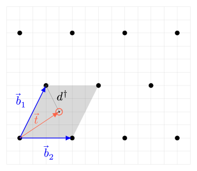
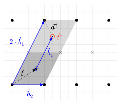
Given the lattice basis $𝐁 : = {𝑏 1, \dots, 𝑏 𝑛}$ , the Search-CVP solver creates sublattices $L (𝐁 *)$ of $L (𝐁)$ using a “dilated” basis
$𝐁 * : = [2 ⃗ 𝑏 1, ⃗ 𝑏 2, \dots, ⃗ 𝑏 𝑛] .$
Since $L (𝐁 *)$ is a subgroup of $L (𝐁)$ , by construction, its quotient group is $L (𝐁) / L (𝐁 *) = {L (𝐁 *), L (𝐁 *) + ⃗ 𝑏 1} ⟹ L (𝐁) = L (𝐁 *) ⨆ (L (𝐁 *) + ⃗ 𝑏 1) ⟹ P (𝐁 *) = P (𝐁) ⨆ (P (𝐁) + ⃗ 𝑏 1) .$

Given that $P (𝐁 *)$ is the disjoint union of $P (𝐁)$ and $P (𝐁) + ⃗ 𝑏 1$ , either $⃗ 𝑡$ or $⃗ 𝑡 + ⃗ 𝑏 1$ must be $𝑑 †$ apart from $L (𝐁 *)$ . (See Fig. 2 for an illustration.) Therefore, the solver can easily maintain the invariant in (19) provided it can decide whether: $Δ (⃗ 𝑡, L (𝐁 *)) = 𝑑 † or Δ (⃗ 𝑡 + ⃗ 𝑏 1, L (𝐁 *)) = 𝑑 † ? (20)$
To decide between the above two cases in (20), the solver invokes $𝜉 1 ⟵$ Decisional-CVP $(𝐁 *, ⃗ 𝑡, 𝑑 †) \in {0, 1}$ to determine if $⃗ 𝑡$ is still $𝑑 †$ apart from $L (𝐁 *)$ ? If $𝜉 1 = 1$ then $Δ (⃗ 𝑡, L (𝐁 *)) = 𝑑 †$ , otherwise $Δ (⃗ 𝑡 + ⃗ 𝑏 1, L (𝐁 *)) = 𝑑 †$ . By updating the target vector to $⃗ 𝑡 * \leftarrow ⃗ 𝑡 + (1 - 𝜉 1) \cdot ⃗ 𝑏 1,$ the solver can maintain the invariant $Δ (⃗ 𝑡 *, L (𝐁 *)) = Δ (⃗ 𝑡, L (𝐁)) = 𝑑 † .$

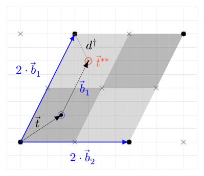
Furthermore, suppose the Search-CVP solver could somehow find the closest vector $⃗ 𝑥 * \in L (𝐁 *)$ to $⃗ 𝑡 *$ , then finding the closest vector $⃗ 𝑥 \in L (𝐁)$ to $⃗ 𝑡$ is easy: $⃗ 𝑥 = ⃗ 𝑥 * - (1 - 𝜉 1) \cdot ⃗ 𝑏 1 .$
The solver repeats the above procedure for all the $𝑛$ basis vectors, $⃗ 𝑏 1, \dots, ⃗ 𝑏 𝑛$ , updating the target vector $⃗ 𝑡$ to $⃗ 𝑡 * \dots *$ using help from Decisional-CVP oracle. At the end of one complete round covering all columns of $𝐁$ , the Search-CVP solver would be left with:
- A sublattice $L (2 𝐁) \subseteq L (𝐁)$ with basis $2 𝐁 = [2 ⃗ 𝑏 1, 2 ⃗ 𝑏 2, \dots, 2 ⃗ 𝑏 𝑛]$
- A displacement vector $⃗ ℎ : = 𝑛 \sum 𝑖 = 1 (1 - 𝜉 𝑖) \cdot ⃗ 𝑏 𝑖 \in L (𝐁)$ where each $𝜉 𝑖 \in {0, 1}$ is the output of invocations to Decisional-CVP oracle, and
- The updated target vector $⃗ 𝑡 * \dots * \leftarrow ⃗ 𝑡 + ⃗ ℎ$ that maintains the invariant $Δ (⃗ 𝑡 * \dots *, 2 𝐁) = Δ (⃗ 𝑡, 𝐁) = 𝑑 † .$
- As before, if the Search-CVP solver could somehow find the closest lattice vector $⃗ 𝑥 * \dots * \in L (2 𝐁)$ to $⃗ 𝑡 * \dots *$ , then the solver can find the closest lattice vector $⃗ 𝑥 \in L (𝐁)$ to $⃗ 𝑡$ as $⃗ 𝑥 = ⃗ 𝑥 * \dots * - ⃗ ℎ \in L (𝐁) .$
Let $𝜆 1 (𝐁)$ be the length of the shortest non-zero vector in $L (𝐁)$ and let $̂ 𝛼 (⃗ 𝑡, 𝐁) : = Δ (⃗ 𝑡, L (𝐁)) 𝜆 1 (𝐁) .$

Before the solver can invoke $𝛼$ -BDD oracle, it must ensure that $̂ 𝛼 (⃗ 𝑡 * \dots *, 𝐁 * \dots *) < 𝛼$ for $𝛼$ -BDD to find the unique solution. Since $𝜆 1 (2 𝐁) = 2 \cdot 𝜆 1 (𝐁)$ while $Δ (⃗ 𝑡, L (𝐁)) = Δ (⃗ 𝑡 * \dots *, L (2 𝐁))$ $⟹$ $𝛼 (⃗ 𝑡 * \dots *, 2 𝐁) = 12 𝛼 (⃗ 𝑡, 𝐁)$ . Therefore, repeating the above procedure $𝑘$ -times results in the updated target vector $⃗ 𝑡 k times ⏞ * \dots *$ with a sublattice basis $2 𝑘 𝐁 = [2 𝑘 ⃗ 𝑏 1, \dots, 2 𝑘 ⃗ 𝑏 𝑛]$ and $𝛼 (⃗ 𝑡 k times ⏞ * \dots *, 2 𝑘 𝐁) = 1 2 𝑘 𝛼 (⃗ 𝑡, 𝐁) .$

Unfortunately, the solver doesn’t know $𝜆 1 (𝐁)$ ! To address that, let $𝐿 = m i n 1 \leq 𝑖 \leq 𝑛 {‖ ⃗ 𝑏 𝑖 ‖}$ be the length of the shortest basis vector of $𝐁$ . By definition, $𝜆 1 (𝐁) \leq 𝐿$ , therefore $Δ (⃗ 𝑡, L (𝐁)) 𝐿 \leq Δ (⃗ 𝑡, L (𝐁)) 𝜆 1 (𝐁) ⟹ 𝑑 † 2 𝑘 \cdot 𝐿 = Δ (⃗ 𝑡 k times ⏞ * \dots *, L (𝐁 k times ⏞ * \dots *)) 2 𝑘 \cdot 𝐿 \leq Δ (⃗ 𝑡 k times ⏞ * \dots *, L (𝐁 k times ⏞ * \dots *)) 2 𝑘 \cdot 𝜆 1 (𝐁) .$

Therefore, to ensure $̂ 𝛼 (⃗ 𝑡 k times ⏞ * \dots *, 2 𝑘 \cdot 𝐁) < 𝛼$ it’s sufficient to iterate the above steps $𝑘$ -times, where $𝑘 \geq ⌈ l o g 2 (𝑑 † 𝛼 \cdot 𝐿) ⌉ (21)$

As proved in the next subsection, Babai’s nearest plane approximation algorithm acts as an $𝛼$ -BDD solver for $𝛼 = 1 1 + 2 𝑛 / 2$ . Substituting this value of $𝛼$ in (21) leads to $𝑘 \geq ⌈ l o g 2 (1 + 2 𝑛 / 2) + l o g 2 (𝑑 † / 𝐿) ⌉ \in 𝑂 (𝑛) .$

Lattice with basis

𝐁 : = [⃗ 𝑏 1, ⃗ 𝑏 2],

target vector

⃗ 𝑡

, and computed minimum distance

𝑑 † = Δ (L (𝐁), ⃗ 𝑡)

Iteration-1: Sublattice with basis

𝐁 * : = [2 ⃗ 𝑏 1, ⃗ 𝑏 2]

has

Δ (L (𝐁 *), ⃗ 𝑡) > 𝑑 †

and requires updating the target vector to

⃗ 𝑡 * \leftarrow ⃗ 𝑡 + ⃗ 𝑏 1

to maintain the invariant

Δ (L (𝐁 *), ⃗ 𝑡 *) = 𝑑 †

Iteration-2: Sublattice with basis

𝐁 * * : = [2 ⃗ 𝑏 1, 2 ⃗ 𝑏 2]

implicitly preserves the invariant

Δ (L (𝐁 * *), ⃗ 𝑡 *) = 𝑑 †

and does not require update to target vector

⃗ 𝑡 *

, therefore

⃗ 𝑡 * * \leftarrow ⃗ 𝑡 *

Two iterations of Search-CVP to Decisional-CVP reduction.

The exact steps of the reduction are described below:

Search-CVP solver via $1 1 + 2 𝑛 / 2$ -BDD

Compute $𝐿 = m i n 1 \leq 𝑖 \leq 𝑛 {‖ ⃗ 𝑏 𝑖 ‖}$

set iteration count $𝑘 = ⌈ l o g 2 (1 + 2 𝑛 / 2) + l o g 2 (𝑑 † / 𝐿) ⌉$

set displacement vector $⃗ ℎ = ⃗ 0 \in L (𝐁)$

for $𝑖 \leftarrow 1 \dots 𝑘$ do

for $𝑗 = 1 \dots 𝑛$ do

Let the basis so far be $𝐁 = [⃗ 𝑏 1, \dots, ⃗ 𝑏 𝑛]$ , update basis: $𝐁 \leftarrow [⃗ 𝑏 1, \dots, ⃗ 𝑏 𝑗 - 1, 2 \cdot ⃗ 𝑏 𝑗, ⃗ 𝑏 𝑗 + 1, \dots, ⃗ 𝑏 𝑛]$

invoke $𝜉 \leftarrow$ Decisional-CVP $(𝐁, ⃗ 𝑡, 𝑑 †)$ and update $⃗ 𝑡 \leftarrow ⃗ 𝑡 + (1 - 𝜉) \cdot ⃗ 𝑏 𝑗 ⃗ ℎ \leftarrow ⃗ ℎ + (1 - 𝜉) \cdot ⃗ 𝑏 𝑗$

compute LLL reduced basis $̃ 𝐁 \leftarrow LLL (𝐁)$ .

invoke $⃗ 𝑥 \leftarrow 𝛼$ -BDD $(̃ 𝐁, ⃗ 𝑡)$ .

return $⃗ 𝑥 - ⃗ ℎ$ .

Note: Even though the BDD oracle is invoked on LLL reduced basis, the closeness of $⃗ 𝑥$ to $⃗ 𝑡$ is independent of the choice of basis.

The next subsection describes Babai’s nearest plane algorithm and proves that it solves $𝛼$ -BDD exactly for $𝛼 < 1 1 + 2 𝑛 / 2$ .

Polynomial time algorithm for $1 1 + 2 𝑛 / 2$ `-BDD` instance

Babai’s nearest plane algorithm is a polynomial time approximation algorithm for CVP. Details of this algorithm for an arbitrary lattice basis $𝐁$ is described below.

(Babai's Nearest Plane Algorithm)

Input: A non-singular lattice basis $𝐁 = {𝑏 𝑖} \in ℤ 𝑛 \times 𝑛$; A target vector $⃗ 𝑡 \in ℚ 𝑛$
Output: $⃗ 𝑥 \in L (𝐁)$; $⃗ 𝑒 \in P (𝐁 ⟂)$ such that $⃗ 𝑡 = ⃗ 𝑥 + ⃗ 𝑒$ where $P (𝐁 ⟂)$ is fundamental domain of Gram-Schmidt orthogonal basis.

The algorithm works by computing the Gram-Schmidt orthogonal basis $𝐁 ⟂ : = [⃗ 𝑏 ⟂ 1, \dots, ⃗ 𝑏 ⟂ 𝑛]$ and progressively projecting the target vector to $⃗ 𝑏 ⟂ 𝑖$ and uses rounding to find a lattice vector “close” to $⃗ 𝑡$ .

In more detail:

Compute Gram-Schmidt orthogonal basis $𝐁 ⟂ : = [⃗ 𝑏 ⟂ 1, \dots, ⃗ 𝑏 ⟂ 𝑛] \leftarrow gso (𝐁) \in ℚ 𝑛 \times 𝑛$

Initialize error term $⃗ 𝑒 \leftarrow ⃗ 𝑡 \in ℚ 𝑛$

Initialize “close” lattice $⃗ 𝑥 \leftarrow ⃗ 0 \in ℤ 𝑛$

for $𝑖 \leftarrow 𝑛 \dots 1$ do

Compute $𝑘 : = ⌊ ⟨ ⃗ 𝑒, ⃗ 𝑏 ⟂ 𝑖 ⟩ ∥ ⃗ 𝑏 ⟂ 𝑖 ∥ 2 ⌉ \in ℤ$

$⃗ 𝑒 \leftarrow ⃗ 𝑒 - 𝑘 \cdot ⃗ 𝑏 𝑖$

$⃗ 𝑥 \leftarrow ⃗ 𝑥 + 𝑘 \cdot ⃗ 𝑏 𝑖$

Return $(⃗ 𝑥, ⃗ 𝑒)$ .

For an arbitrary (bad) basis $𝐁$ , this algorithm does not guarantee that its output will be a known bounded approximation to Search-CVP. If $𝐁$ is an LLL reduced basis, then one can show that $⃗ 𝑥$ is guaranteed to be at a distance that’s at most $2 𝑛 / 2$ times the optimal. That is, if the optimal solution to Search-CVP $(𝐁, ⃗ 𝑡)$ is $⃗ 𝑥 †$ then $‖ ⃗ 𝑥 - ⃗ 𝑡 ‖ \leq 2 𝑛 / 2 \cdot Δ (⃗ 𝑡, L (𝐁)) = 2 𝑛 / 2 \cdot ‖ ⃗ 𝑥 † - ⃗ 𝑡 ‖ .$

More generally, suppose Babai’s nearest plane algorithm returns $⃗ 𝑥 \in L (𝐁)$ that’s a $𝛾 (𝑛)$ approximation to Search-CVP, i.e., $‖ ⃗ 𝑥 - ⃗ 𝑡 ‖ \leq 𝛾 (𝑛) \cdot Δ (⃗ 𝑡, L (𝐁))$ . For an $𝛼$ -BDD problem instance, we wish to derive the range of values of $𝛼 \in [0, 12)$ for which Babai’s nearest plane algorithm can solve Search-CVP exactly in polynomial time.

By triangle inequality $‖ ⃗ 𝑥 - ⃗ 𝑥 † ‖ = ‖ ⃗ 𝑥 - ⃗ 𝑡 + ⃗ 𝑡 - ⃗ 𝑥 † ‖ \leq ‖ ⃗ 𝑥 - ⃗ 𝑡 ‖ + ‖ ⃗ 𝑥 † - ⃗ 𝑡 ‖ (22)$

By assumption, for an $𝛼$ -BDD instance, $‖ ⃗ 𝑥 † - ⃗ 𝑡 ‖ < 𝛼 \cdot 𝜆 1$ . Furthermore, the nearest plane algorithm guarantees that $‖ ⃗ 𝑥 - ⃗ 𝑡 ‖ < 𝛾 (𝑛) \cdot Δ (⃗ 𝑡, L (𝐁))$ , which again by $𝛼$ -BDD promise implies $‖ ⃗ 𝑥 - ⃗ 𝑡 ‖ < 𝛾 (𝑛) \cdot 𝛼 \cdot 𝜆 1$ . Therefore by (22): $‖ ⃗ 𝑥 - ⃗ 𝑥 † ‖ \leq 𝛾 (𝑛) \cdot Δ (⃗ 𝑡, L (𝐁)) + 𝛼 \cdot 𝜆 1 \leq 𝛾 (𝑛) \cdot 𝛼 \cdot 𝜆 1 + 𝛼 \cdot 𝜆 1 = (1 + 𝛾 (𝑛)) \cdot 𝛼 \cdot 𝜆 1 .$

On the other hand, if $⃗ 𝑥$ and $⃗ 𝑥 †$ are distinct, then $𝜆 1 \leq ‖ ⃗ 𝑥 - ⃗ 𝑥 † ‖$ , and hence $𝜆 1 \leq (1 + 𝛾 (𝑛)) \cdot 𝛼 \cdot 𝜆 1 ⟹ 𝛼 \geq 1 1 + 𝛾 (𝑛) .$

In other words, if $𝛼 \geq 1 1 + 𝛾 (𝑛)$ then Babai’s nearest plane algorithm is likely to output a lattice vector that’s not necessarily the optimal $⃗ 𝑥 †$ . Conversely, if $𝛼 < 1 1 + 𝛾 (𝑛)$ then $⃗ 𝑥$ and $⃗ 𝑥 †$ cannot be distinct and Babai’s nearest plane algorithm will output the optimal solution to Search-CVP! For example, if $𝐁$ is an LLL reduced basis, then for $𝛼 < 1 1 + 2 𝑛 / 2$ , the nearest plane algorithm will output the optimal solution to Search-CVP.

Sanity Check: If $𝛾 (𝑛) = 1$ then the result above requires $𝛼 < 12$ for a unique solution, which matches with the uniqueness requirement for $𝛼$ -BDD.

D. Aharonov and O. Regev, “Lattice problems in $𝖭 𝖯 \cap 𝖼 𝗈 𝖭 𝖯$ ,” in Journal of the ACM (JACM), Volume 52, Issue 5., Pages 749 - 765. ↩
S. Khot, “Hardness of approximating the shortest vector problem in lattices,” in Journal of the ACM (JACM), Volume 52, Issue 5., Pages 789 - 808 ↩
I. Haviv and O. Regev, “Tensor-based Hardness of the Shortest Vector Problem to within Almost Polynomial Factors,” in Theory of Computing Journal, Volume 8 (2012), Pages 513 - 531. ↩
Y. Liu, V. Lyubashevsky and D. Micciancio, “On Bounded Distance Decoding for General Lattices,” in 9th International Workshop on Approximation Algorithms for Combinatorial Optimization Problems, APPROX 2006 and 10th International Workshop on Randomization and Computation, RANDOM 2006, Barcelona, Spain, August 28-30, 2006. Pages 450 - 461 ↩ ↩²
H. Bennett and C. Peikert, “Hardness of Bounded Distance Decoding on Lattices in $ℓ 𝑝$ Norms,” in 35th Computational Complexity Conference (CCC 2020). Available Online ↩
D. Micciancio and S. Goldwasser, “Complexity of Lattice Problems: A Cryptographic Perspective,” Springer, New York, NY., 2002, DOI: https://doi.org/10.1007/978-1-4615-0897-7 ↩ ↩²
P. v. E. Boas, “Another $𝖭 𝖯$ -complete partition problem and the complexity of computing short vectors in a lattice,” Technical Report, 1981. Available Online ↩
M. R. Garey and D. S. Johnson, “Computers and Intractability: A Guide to the Theory of NP-Completeness,” W. H. Freeman, 1979. ↩
K. Kreuzer and T. Nipkow, “Verification of NP-hardness Reduction Functions for Exact Lattice Problems” in the Proceedings of CADE 29: 29th International Conference on Automated Deduction, Rome, Italy, July 1–4, 2023. Available Online ↩
R. Kannan, “Minkowski’s convex body theorem and integer programming,” Mathematics of Operations Research, 12(3), 1987. Pages 415–440 ↩ ↩²
N. Stephens-Davidowitz, “Search-to-Decision Reductions for Lattice Problems with Approximation Factors (Slightly) Greater Than One,” in Approximation, Randomization, and Combinatorial Optimization, Algorithms and Techniques (APPROX/RANDOM 2016), Article No. 19; Pages 19:1–19:18 ↩

SVP and CVP Problem Instances

The Closest Vector Problem

(Distance from a Lattice, Closest Vector)

Exact Closest Vector Problem (CVP)

(Search-CVP)

(Opt-CVP)

(Decisional-CVP)

(Bounded distance Decoding, 𝛼-BDD)

Approximate Closest Vector Problem (𝛾-CVP)

(Approx-CVP𝛾)

(GapCVP𝛾)

(Gap Reductions)

Reductions among exact problems

Decisional-CVP is 𝖭𝖯-Complete

(Subset-Sum)

(Subset-Sum ⪯ Decisional-CVP)

Decisional-SVP|ℓ∞ is 𝖭𝖯-Complete

Subset-Sum ⪯ 2-Partition

(2-Partition)

(Subset-Sum ⪯ 2-Partition)

2-Partition ⪯ ℓ∞-Bounded Homogeneous Linear Equation (BHLE)

(ℓ∞-Bounded Homogeneous Linear Equation)

(↪𝑎∈ 2-Partition ⟹𝜉(↪𝑎)∈ BHLE)

(Unique Bit Decomposition)

(𝜉(↪𝑎)∈ BHLE ⟹↪𝑎∈ 2-Partition)

BHLE ⪯ Decisional-SVP|ℓ∞

((⃗𝑎,𝜅)∈𝖡𝖧𝖫𝖤⟹𝜁(⃗𝑎,𝜅)∈Decisional-SVP)

(∃(⃗𝑎,𝜅):𝜁(⃗𝑎,𝜅)∈Decisional-SVP⟹(⃗𝑎,𝜅)∈𝖡𝖧𝖫𝖤)

Search-CVP reduces to Decisional-CVP

(Opt-CVP ⪯ Decisional-CVP)

Opt-CVP Solver

(CVP Exhaustive Search)

Search-CVP reduces to 𝛼-BDD

(Search-CVP[Decisional-CVP] ⪯𝛼-BDD)

Search-CVP solver via 11+2𝑛/2-BDD

Polynomial time algorithm for 11+2𝑛/2-BDD instance

(Babai's Nearest Plane Algorithm)

Comments

(Bounded distance Decoding, $𝛼$ -BDD)

Approximate Closest Vector Problem ( $𝛾$ -CVP)

(Approx-CVP $𝛾$ )

(GapCVP $𝛾$ )

Decisional-CVP is $𝖭 𝖯$ -Complete

(Subset-Sum $⪯$ Decisional-CVP)

Decisional-SVP $| ℓ \infty$ is $𝖭 𝖯$ -Complete

Subset-Sum $⪯$ $2$ -Partition

( $2$ -Partition)

(Subset-Sum $⪯$ $2$ -Partition)

$2$ -Partition $⪯$ $ℓ \infty$ -Bounded Homogeneous Linear Equation (BHLE)

( $ℓ \infty$ -Bounded Homogeneous Linear Equation)

( $↪ 𝑎 \in$ $2$ -Partition $⟹ 𝜉 (↪ 𝑎) \in$ BHLE)

( $𝜉 (↪ 𝑎) \in$ BHLE $⟹ ↪ 𝑎 \in$ $2$ -Partition)

BHLE $⪯$ Decisional-SVP $| ℓ \infty$

( $(⃗ 𝑎, 𝜅) \in 𝖡 𝖧 𝖫 𝖤 ⟹ 𝜁 (⃗ 𝑎, 𝜅) \in Decisional-SVP$ )

( $\exists (⃗ 𝑎, 𝜅) : 𝜁 (⃗ 𝑎, 𝜅) \in Decisional-SVP ⟹ (⃗ 𝑎, 𝜅) \in 𝖡 𝖧 𝖫 𝖤$ )

(Opt-CVP $⪯$ Decisional-CVP)

`Search-CVP` reduces to $𝛼$ `-BDD`

(Search-CVP^{[Decisional-CVP]} $⪯ 𝛼$ -BDD)

Search-CVP solver via $1 1 + 2 𝑛 / 2$ -BDD

Polynomial time algorithm for $1 1 + 2 𝑛 / 2$ `-BDD` instance