Lattices of Cryptography — Basic Results

Table of Contents

Basis Independent Characterization
Basis Dependent Characterization
- Fundamental Parallelepiped
Length of Lattice Vectors
Equivalence of definitions

This post is a grab bag of basic definitions and elementary results related to unstructured lattices. See ¹ for a more condensed version of similar topics or ² for a more detailed and advanced algebraic treatment.

Basis Independent Characterization

A lattice $L$ is a discrete additive subgroup of $ℝ 𝑛$ , that is,

$L$ inherits the additive group structure of $ℝ 𝑛$ ,
$L$ is equipped with a notion of distance, (or equivalently, a inner product $⟨ \cdot, \cdot ⟩ : L \times L \mapsto ℝ$ ), and
there exits a fixed non-zero radius $𝜖$ (see Fig. 1), such that the open ball $𝔹 (⃗ 𝑥, 𝜖) : = {𝑦 \in ℝ 𝑛 : ‖ 𝑥 - 𝑦 ‖ < 𝜖}$ centered at $⃗ 𝑥 \in L$ , contains no other elements of $L$ , i.e., $\exists 𝜖 > 0, \forall ⃗ 𝑥 \in L : 𝔹 (⃗ 𝑥, 𝜖) \cap L = {⃗ 𝑥} . (1)$

Lattices can be defined more broadly as finitely generated modules over an integral domain, embedded into a vector space over its fraction field! But for the purposes of this post, the above limited definition is sufficient. Full generality, however, brings with itself full complexity, which does not always aid in understanding.

Since $L$ is an additive subgroup of $ℝ 𝑛$ , translations of $L$ by an arbitrary vector $⃗ 𝑣 \in ℝ 𝑛$ forms the usual equivalence class of cosets defined by $[⃗ 𝑣] : = ⃗ 𝑣 + L = {⃗ 𝑣 + ⃗ 𝑥 : ⃗ 𝑥 \in L} \in ℝ 𝑛 / L .$

By definition, two arbitrary vectors $⃗ 𝑥, ⃗ 𝑦 \in ℝ 𝑛$ belong to the same coset, if and only if $⃗ 𝑥 - ⃗ 𝑦 \in L$ . Any set $̂ P \subset ℝ 𝑛$ that contains exactly one representative element $⃗ 𝑣$ from each coset $[⃗ 𝑣] \in ℝ 𝑛 / L$ is called a strict fundamental domain of $L$ , and is defined as

̂ P : = ⋃ [⃗ 𝑣] \in ℝ 𝑛 / L ⃗ 𝑣 . (2)

Since the choice of representative $⃗ 𝑣 \in [⃗ 𝑣]$ is arbitrary, $̂ P$ is not uniquely determined. However, $ℝ 𝑛 / L$ partitions $ℝ 𝑛$ into its cosets, therefore translations of any given $̂ P$ by the lattice vectors tiles the entire $ℝ 𝑛$ without overlap, i.e.,

⋃ ⃗ 𝑥 \in L (̂ P + ⃗ 𝑥) = ℝ 𝑛 and \forall ⃗ 𝑥, ⃗ 𝑦 \in L, ⃗ 𝑥 \neq ⃗ 𝑦 : (̂ P + ⃗ 𝑥) ⋂ (̂ P + ⃗ 𝑦) = \emptyset .

The covolume (sometimes also called volume) is the volume of any of its strict fundamental domains (i.e., a measure of its size). For any translation invariant measure, like the Lebesgue measure, the covolume is independent of the choice of representatives used to define $̂ P$ .

Basis Dependent Characterization

The characterization of a lattice so far has been entirely basis independent. This is ideal for exploring algebraic and topological properties of lattices, however, it’s not very useful for computational purposes. For that, the following basis dependent characterization is more suitable.

(Lattice with basis)

A lattice $L$ of rank $𝑚$ and dimension $𝑛$ is the set of all possible integer linear combinations of $𝑚$ linearly independent (over $ℝ$ ) vectors $⃗ 𝑏 1, \dots, ⃗ 𝑏 𝑚 \in ℝ 𝑛$ (where $𝑚 \leq 𝑛$ ), i.e.,

L : = {𝑧 1 ⃗ 𝑏 1 + \dots + 𝑧 𝑚 ⃗ 𝑏 𝑚 : 𝑧 𝑖 \in ℤ} \subseteq ℝ 𝑛 . (3)

Since ${⃗ 𝑏 𝑖}$ s are linearly independent, its convenient to treat them as basis vectors of $L$ and represent them as columns of a matrix $𝐁 : = ⎛ ⎜ ⎜ ⎜ ⎜ ⎝ | | ⃗ 𝑎 1 \dots ⃗ 𝑎 𝑚 | | ⎞ ⎟ ⎟ ⎟ ⎟ ⎠ \in ℝ 𝑛 \times 𝑚 .$

To emphasize that $L$ is generated by $𝐁$ , we will use the notation $L (𝐁)$ . Furthermore, bold uppercase letters written as $𝐂 : = {⃗ 𝑐 1, \dots, ⃗ 𝑐 𝑚}$ will be treated both as a set as well as a matrix whose columns have some pre-prescribed ordering.

A few additional definitions are listed below, which should largely be familiar to most readers:

Dimension: The dimension of $L \subseteq ℝ 𝑛$ is the dimension of the ambient vector space $ℝ 𝑛$ , which is $𝑛$ .
Rank: Algebraically, a lattice is also a free $ℤ$ -module, and the rank of $L$ is the rank of the corresponding $ℤ$ -module. Since the rank of a free module is independent of the choice of its basis, rank of $L$ is well defined and independent of the choice of its basis. When a basis $𝐁 \in ℝ 𝑛 \times 𝑚$ is explicitly given, the rank of $L (𝐁)$ is the number of linearly independent columns of $𝐁 .$
Full Rank: A lattice whose rank is same as its dimension (that is, $𝑚 = 𝑛$ ) is called a full rank lattice.
Span: The span of a lattice $L (𝐁)$ is the span of $𝐁$ as a $ℝ$ -vector space, i.e., $span ℝ (L (𝐁)) : = span ℝ (𝐁) = {𝐁 \cdot ⃗ 𝑦 : 𝑦 \in ℝ 𝑚}$

When do two bases $𝐁 1$ and $𝐁 2$ generate the same lattice? The following theorem characterizes this precisely:

(Basis Equivalence)

Let $𝐁 1, 𝐁 2 \in ℝ 𝑛 \times 𝑚$ be two matrices with column rank $𝑚 \leq 𝑛$ . Then, $𝐁 1$ and $𝐁 2$ generate the same lattice $L$ if and only if there exists an integer matrix $𝐔 \in ℤ 𝑚 \times 𝑚$ such that $𝐁 2 = 𝐁 1 \cdot 𝐔 and d e t (𝐔) = \pm 1 .$

We first show that if $L (𝐁 2) = L (𝐁 1)$ then $\exists 𝐔 \in ℤ 𝑚 \times 𝑚$ such that $d e t (𝐔) = 1$ and $𝐁 2 = 𝐁 1 \cdot 𝐔$ .

( $\Rightarrow$ ):

Since $L (𝐁 2) = L (𝐁 1)$ , each column ${𝑏 1, \dots, 𝑏 𝑚}$ of $𝐁 2$ is also an element of $L (𝐁 1)$ . Therefore, for every $𝑖$ -th column of $𝐁 2$ , there exists $⃗ 𝑢 𝑖 \in ℤ 𝑚$ , such that $𝑏 𝑖 = 𝐁 1 \cdot ⃗ 𝑢 𝑖$ . If we define $𝐔$ to be the matrix whose columns are $⃗ 𝑢 𝑖$ s, then $𝐔 \in ℤ 𝑚 \times 𝑚$ satisfies the relation: $𝐁 2 = 𝐁 1 \cdot 𝐔 .$

By a similar argument, there exists $𝐕 \in ℤ 𝑚 \times 𝑚$ such that $𝐁 1 = 𝐁 2 \cdot 𝐕 .$

Therefore, $𝐁 2 = (𝐁 2 \cdot 𝐕) \cdot 𝐔 = 𝐁 2 \cdot (𝐕 \cdot 𝐔) ⟹ 𝐁 2 \cdot (𝐈 𝑚 - 𝐕 \cdot 𝐔) = ⃗ 0,$ where $𝐈 𝑚 \in ℤ 𝑚 \times 𝑚$ is the identity matrix, and $⃗ 0 \in ℝ 𝑛$ is the all zero vector.

Since columns of $𝐁 𝑖$ s are assumed to be linearly independent, the linear transformation $⃗ 𝑧 \mapsto 𝐁 𝑖 \cdot ⃗ 𝑧$ is injective, i.e., $𝐁 𝑖 \cdot ⃗ 𝑧 = 0 ⟺ ⃗ 𝑧 = ⃗ 0$ . Therefore, $𝐁 2 \cdot (𝐈 𝑚 - 𝐕 \cdot 𝐔) = ⃗ 0 ⟹ (𝐈 𝑚 - 𝐕 \cdot 𝐔) = ⃗ 0 ⟹ 𝐕 \cdot 𝐔 = 𝐈 𝑚 .$

That means, $𝐔$ and $𝐕$ are inverses of each other! However, $𝐔$ and $𝐕$ are both integer matrices, and they can be inverses of each other if and only if $d e t (𝐔) = d e t (𝐕) = \pm 1 .$

Conversely, if $𝐔 \in ℤ 𝑚 \times 𝑛$ is such that $𝐁 2 = 𝐁 1 \cdot 𝐔$ and $d e t (𝐔) = \pm 1$ , then we need to show that $L (𝐁 2) = L (𝐁 1)$ .

( $\Leftarrow$ ):

Given that $𝐔$ is an integer matrix, $𝐔 \cdot ℤ 𝑚 \subseteq ℤ 𝑚$ . Therefore, $L (𝐁 2) = 𝐁 2 \cdot ℤ 𝑚 = (𝐁 1 \cdot 𝐔) \cdot ℤ 𝑚 = 𝐁 1 \cdot (𝐔 \cdot ℤ 𝑚) \subseteq 𝐁 1 \cdot ℤ 𝑚 = L (𝐁 1) .$

Since $d e t (𝐔) = \pm 1$ , $𝐔$ is non-singular and $𝐔 - 1$ has integer entries (because $1 d e t (𝐔) = \pm 1$ ). Therefore, using the relation $𝐁 1 = 𝐁 2 \cdot 𝐔 - 1$ and arguments similar as before, we get $L (𝐁 1) = 𝐁 1 \cdot ℤ 𝑚 = (𝐁 2 \cdot 𝐔 - 1) \cdot ℤ 𝑚 = 𝐁 2 \cdot (𝐔 - 1 \cdot ℤ 𝑚) \subseteq 𝐁 2 \cdot ℤ 𝑚 = L (𝐁 2) .$

Since $L (𝐁 2) \subseteq L (𝐁 1)$ and $L (𝐁 1) \subseteq L (𝐁 2) ⟹ L (𝐁 1) = L (𝐁 2) .$

Integer matrices whose inverse also happen to be an integer matrix have a special name:

(Unimodular Matrix)

An integer matrix $𝐔 \in ℤ 𝑚 \times 𝑚$ is called Unimodular if $d e t (𝐔) = \pm 1 .$

Since the determinant of $𝐔$ is $\pm 1$ , and the $(𝑖, 𝑗)$ -th cofactor entry of an integer matrix is always an integer, inverse of $𝐔$ exists and has integer entries, that is, $𝐔 - 1 \in ℤ 𝑚 \times 𝑚$ . Furthermore, if $𝐔$ and $𝐕$ are unimodular and have the same dimension, then so is $𝐔 \cdot 𝐕$ because $d e t (𝐔 \cdot 𝐕) = d e t (𝐔) d e t (𝐕) = \pm 1 .$

To summarize, unimodular matrices form a group under usual matrix multiplication. This group is called General Linear Group over integers and is denoted by $G L 𝑚 (ℤ)$ . Unimodular matrices whose determinant is $+ 1$ forms a subgroup of $G L 𝑚 (ℤ)$ called the Special Linear Group over integers and is denoted by $S L 𝑚 (ℤ)$ .

While lattices, in general, are defined over reals, for computational problems, only lattices with integer basis vectors (i.e., $𝐁 \in ℤ 𝑛 \times 𝑚 \subseteq ℝ 𝑛 \times 𝑚$ ) are of cryptographic interest. Furthermore, the number of bits needed to represent $𝐁$ is assumed to be a fixed polynomial in the dimension $𝑛$ . This restriction is important for understanding the role of dimension in solving lattice problems. In this post, such lattices are called integral lattices.

⚠️ The definition of integral lattices in this post is different from the standard definition (², Lecture 2). In the standard literature, integral lattices are defined more broadly and are not restricted to integer valued basis vectors. In fact, the only requirement for a lattice to be integral is that $\forall ⃗ 𝑥, ⃗ 𝑦 \in L : ⟨ ⃗ 𝑥, ⃗ 𝑦 ⟩ \in ℤ .$ While the definition used in this post trivially satisfies this definition, its not complete. This discrepancy, however, is of no consequence for computational purposes.

Fundamental Parallelepiped

Rank and dimension are crude invariants of a lattice. A more fine-grained invariant is the covolume of a fundamental parallelepiped, which is defined next.

(Fundamental Parallelepiped)

Given a basis $𝐁 : = {⃗ 𝑏 1, \dots, ⃗ 𝑏 𝑚} \in ℝ 𝑛 \times 𝑚$ , the fundamental parallelepiped $P (𝐁)$ is the set of points in $ℝ 𝑛$ that are generated by taking fractional linear combination of the basis vectors, i.e.,

P (𝐁) : = {𝑡 1 ⃗ 𝑏 1 + \dots + 𝑡 𝑚 ⃗ 𝑏 𝑚 : 0 \leq 𝑡 𝑖 < 1; 𝑡 𝑖 \in ℝ} . (4)

The covolume (also called determinant or just volume) of $L (𝐁)$ is the volume of the fundamental parallelepiped $P (𝐁)$ , which can be computed from the Gram matrix $𝐁 ⊤ 𝐁$ as:

c o v o l (L) = c o v o l (P (𝐁)) = \sqrt 𝐁 ⊤ 𝐁 > 0 . (5)

Same lattice with different bases and distinctly shaped parallelepiped.

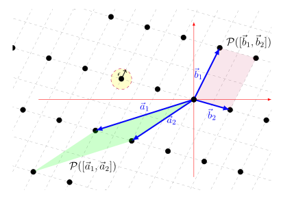
In Fig. 1, the region shaded in green is the fundamental parallelepiped associated with the basis vectors $𝐁 1 : = {⃗ 𝑎 1, ⃗ 𝑎 2}$ . Similarly, the region shaded in purple is also the fundamental parallelepiped, albeit associated with $𝐁 2 : = {⃗ 𝑏 1, ⃗ 𝑏 2}$ . So, even though a lattice is independent of its basis, the shape of a fundamental parallelepiped is not.

However, in spite of this superficial difference, the fundamental parallelepiped for any basis $𝐁$ has two remarkable properties:

$P (𝐁)$ does not contain any non-zero lattice point, and
The covolume of $L$ is independent of the choice of the basis.

The next two lemmas make these observations precise:

Let $L$ be a lattice of rank $𝑚$ and let $𝐂 : = {⃗ 𝑐 1, \dots, ⃗ 𝑐 𝑚 : ⃗ 𝑐 𝑖 \in L}$ be $𝑚$ linearly independent elements of $L$ . Then, $𝐂$ forms a basis of $L,$ if and only if $P (𝐂) \cap L = {⃗ 0} .$

( $\Rightarrow$ ): If $𝐂$ is a basis of $L ⟹ P (𝐁) \cap L = {⃗ 0} .$

By definition, $P (𝐂)$ is the $ℝ$ -span of columns of $𝐂$ restricted to the half-open set $[0, 1)$ . The only integer in this half-open set is $0$ , therefore, $P (𝐂) \cap L = {𝐂 \cdot ⃗ 0} = {⃗ 0} .$

( $\Leftarrow$ ): If $𝐂 \subseteq L$ and $P (𝐂) \cap L = {⃗ 0} ⟹ 𝐂$ is a basis of $L .$

Since the rank of $L$ is $𝑚$ , and $⃗ 𝑐 1, \dots, ⃗ 𝑐 𝑚$ are linearly independent, each lattice vector $⃗ 𝑥 \in L$ can be trivially written as an $ℝ$ -linear combination of $⃗ 𝑐 𝑖$ s, that is: $\forall ⃗ 𝑥 \in L, \exists 𝑟 1, \dots, 𝑟 𝑚 \in ℝ : ⃗ 𝑥 = 𝑟 1 ⃗ 𝑐 1 + \dots + 𝑟 𝑚 ⃗ 𝑐 𝑚 .$ Given that $𝑟 𝑖$ s are real, they can be written as sum of integral and fractional parts as: $𝑟 𝑖 = ⌊ 𝑟 𝑖 ⌋ + ⟦ 𝑟 𝑖 ⟧$ where $⌊ 𝑟 𝑖 ⌋ \in ℤ$ and $⟦ ⃗ 𝑟 𝑖 ⟧ : = ⃗ 𝑟 𝑖 - ⌊ ⃗ 𝑟 𝑖 ⌋ \in [0, 1) 𝑛 \subseteq ℝ 𝑛$ . Therefore, $⃗ 𝑥 = 𝑚 \sum 𝑖 = 1 (⌊ 𝑟 𝑖 ⌋ + ⟦ 𝑟 𝑖 ⟧) \cdot ⃗ 𝑐 𝑖 = 𝑚 \sum 𝑖 = 1 ⌊ 𝑟 𝑖 ⌋ \cdot ⃗ 𝑐 𝑖 + 𝑚 \sum 𝑖 = 1 ⟦ 𝑟 𝑖 ⟧ \cdot ⃗ 𝑐 𝑖$ and $⃗ 𝑥 - (𝑚 \sum 𝑖 = 1 ⌊ 𝑟 𝑖 ⌋ \cdot ⃗ 𝑐 𝑖) = (𝑚 \sum 𝑖 = 1 ⟦ 𝑟 𝑖 ⟧ \cdot ⃗ 𝑐 𝑖) \in P (𝐂) .$

By assumption, each $⃗ 𝑐 𝑖$ is an element of $L$ , which means $(⃗ 𝑥 - \sum 𝑚 𝑖 = 1 ⌊ 𝑟 𝑖 ⌋ \cdot ⃗ 𝑐 𝑖) \in L$ . On the other hand, the right hand side of equation above is an element of $P (𝐂)$ . But by assumption, $P (𝐂) \cap L = {⃗ 0}$ , so the equality can only hold if $⃗ 𝑥 - 𝑚 \sum 𝑖 = 1 ⌊ 𝑟 𝑖 ⌋ \cdot ⃗ 𝑐 𝑖 = ⃗ 0 .$

Therefore, each $𝑟 𝑖$ must be an integer and every $⃗ 𝑥$ can be written as an integer linear combination of columns of $𝐂$ . In short, $𝐂$ is a basis of $L .$

Note: For the previous lemma to hold, it’s crucial that $⃗ 𝑐 𝑖$ s are a priori known to be elements of $L$ . If $𝐂$ is any arbitrary linearly independent set in $ℝ 𝑛$ that satisfies $P (𝐂) \cap L = {⃗ 0}$ , then such a $𝐂$ will not form a basis of $L$ .

The most remarkable property of a fundamental parallelepiped is that its covolume is independent of the choice of the basis.

(Volume Invariance)

The covolume of a lattice $L$ is independent of the choice of its basis. That is, if $𝐁 1, 𝐁 2 \in ℝ 𝑛 \times 𝑚$ are two different bases of $L$ , then $c o v o l (P (𝐁 1)) = c o v o l (P (𝐁 2)) .$

Since $𝐁 1$ and $𝐁 2$ both generate $L$ , by the Basis Equivalence Theorem, there exists $𝐔 \in ℤ 𝑚 \times 𝑚$ with $d e t (𝑈) = 1$ such that $𝐁 1 = 𝐁 2 𝐔 .$ Therefore, $d e t (𝐁 ⊤ 1 \cdot 𝐁 1) = d e t (𝐔 ⊤ 𝐁 ⊤ 2 \cdot 𝐁 2 𝐔) = d e t (𝐔 ⊤) d e t (𝐁 ⊤ 2 \cdot 𝐁 2) d e t (𝐔)) = d e t (𝐁 ⊤ 2 \cdot 𝐁 2)$ and $c o v o l (P (𝐁 1)) = c o v o l (P (𝐁 2)) .$

Notice that by construction, the fundamental parallelepiped $P (𝐁)$ is also a strict fundamental domain $̂ P$ (2) whose the coset representatives form a connected convex set. $P (𝐁)$ is connected because the half-open unit interval $[0, 1)$ is connected. It’s convex because if $⃗ 𝑥$ and $⃗ 𝑦$ are elements of $P (𝐁)$ , then $\forall 𝑡 \in [0, 1] \subseteq ℝ : 𝑡 \cdot ⃗ 𝑥 + (1 - 𝑡) \cdot ⃗ 𝑦 \in P (𝐁) .$

Length of Lattice Vectors

Since lattice points form a repeated pattern in $ℝ 𝑛$ , each lattice vector $⃗ 𝑥 \in L$ can be collected into an $𝑛$ -dimensional spherical shell, where each shell contains vectors of the same length. Let $S 𝑗 \subseteq L$ denote the $𝑗$ -th shell and $𝜈 𝑗$ be its radius. Assuming the index $𝑗$ is chosen such that $𝜈 0 = 0$ and $𝜈 𝑗 - 1 < 𝜈 𝑗$ then, the following strict ordering of $𝜈 𝑗$ s is a lattice invariant:

𝜈 0 < \dots < 𝜈 𝑗 - 1 < 𝜈 𝑗 < 𝜈 𝑗 + 1 < \dots < \infty .

For all lattices, $S 0 = {⃗ 0}$ and is called the trivial or zero shell and $S 𝑗$ for $𝑗 > 0$ is called non-trivial or non-zero shell.

Given this setup, there are three natural computational questions one can ask. (See also the aside on bounds of $S 𝑗$ .)

Given an index $𝑗$ , and a lattice $L (𝐁)$ specified by an integral basis $𝐁 \in ℤ 𝑛 \times 𝑚$ , find an element of $S 𝑗$ . For example, when $𝑗 = 0$ it’s trivial to find an element of $S 0$ , since $S 0 = {⃗ 0}$ . But what about finding an element of $S 1$ or $S 13$ ? Does the difficulty depend upon the index $𝑗$ ? Does it depend on the choice of $𝐁$ ?
Given $𝑗$ and $L (𝐁)$ as before, compute the value of $𝜈 𝑗$ . Here, the problem is not to explicitly find a lattice vector but to only compute the radius $𝜈 𝑗$ . Indeed, if one can find an element $⃗ 𝑥 \in S 𝑗$ , then one can trivially compute $𝜈 𝑗 = ‖ ⃗ 𝑥 ‖$ . However, there might be other “short cuts” that directly computes $𝜈 𝑗$ without ever explicitly finding an element of $S 𝑗$ .
Given a lattice vector $⃗ 𝑥 \in L (𝐁)$ find its position $𝑗$ in the partial order, i.e., find $𝑗$ such that $‖ ⃗ 𝑥 ‖ = 𝜈 𝑗 .$

When the rank of $L$ is large, solving any of these three problems is computationally challenging. Cryptographically, however, the most relevant problem is to find an element of $S 1$ — which is also called the shortest vector problem. Surprisingly, it is not only hard to find a non-zero shortest vector, but also hard to find even an “approximately short” vector in $L$ .

The next few subsections make these notions precise.

In the rest of this post, as is the case in general literature, shortest vector will always mean shortest non-zero vector.

(Bounds on the cardinality of

S 𝑗

)

For a full-rank lattice $L$ , what are the upper and lower bounds on the cardinality of $S 1$ (and more generally $S 𝑗$ )? Let $𝜏 𝑛$ denote the cardinality of $S 1$ and $𝜏 (𝑗) 𝑛$ denote the cardinality of $S 𝑗$ .

First notice that the cardinality of any non-zero $S 𝑗$ is always even, so a trivial lower bound is $2$ . This is because if $⃗ 𝑥 \in S 𝑗$ then by definition $⃗ 𝑥 \neq ⃗ 0 \in S 0$ , which means $⃗ 𝑥 \neq - ⃗ 𝑥$ . However, for all $⃗ 𝑥$ , $‖ ⃗ 𝑥 ‖ = ‖ - ⃗ 𝑥 ‖$ , therefore if $⃗ 𝑥$ is an element of $S 𝑗$ , then so is $- ⃗ 𝑥$ , and hence the cardinality of $S 𝑗$ is even!

Surprisingly, for integral lattices, this lower bound is also sharp. That is, for every $𝐽 2$ where $𝐽 \in ℤ$ , there exists a $𝑛$ -dimensional lattice where each shell $S 𝑗$ for $𝑗 \in {1, \dots, 𝐽}$ contains only $2$ lattice points! To see why, let $𝑀 \in ℤ$ be such that $𝑀 > 𝐽$ , and consider the integral lattice generated by the basis:

𝐁 𝑀 : = {⃗ 𝑒 1, 𝑀 ⃗ 𝑒 2, \dots, 𝑀 ⃗ 𝑒 𝑛} \in ℤ 𝑛 \times 𝑛

where $⃗ 𝑒 𝑖$ s are the standard $𝑛$ -dimensional basis vectors.

Claim: For $L (𝐁 𝑀)$ , the first $𝐽$ non-zero shell radii $𝜈 𝑗 = 𝑗$ and $S 𝑗 = {\pm 𝑗 \cdot ⃗ 𝑒 1}$ .

Proof: By definition, every lattice vector $⃗ 𝑥 \in L (𝐁 𝑀)$ can be written as $⃗ 𝑥 = 𝑧 1 \cdot ⃗ 𝑒 1 + 𝑀 \cdot (\sum 𝑛 𝑖 = 2 𝑧 𝑖 \cdot ⃗ 𝑒 𝑖)$ , where $𝑧 𝑖 \in ℤ$ . Consider $𝐽$ lattice vectors $⃗ 𝑦 𝑗$ s generated by setting $𝑧 1 = 𝑗$ for $𝑗 = 1, \dots, 𝐽$ and $𝑧 2 = \dots = 𝑧 𝑛 = 0$ , that is, $⃗ 𝑦 𝑗 : = 𝑗 \cdot ⃗ 𝑒 1$ . Then $‖ ⃗ 𝑦 𝑗 ‖ = ‖ 𝑗 \cdot ⃗ 𝑒 1 ‖ = 𝑗$ .

For an arbitrary vector $⃗ 𝑥 \in L (𝐁 𝑀)$ , it’s length can be written as $‖ ⃗ 𝑥 ‖ 2 = 𝑧 21 + 𝑀 2 (𝑛 \sum 𝑖 = 2 𝑧 2 𝑖) = 𝑧 21 + 𝑀 2 \cdot 𝑍 where 𝑍 : = 𝑛 \sum 𝑖 = 2 𝑧 2 𝑖 \geq 0 .$

Suppose for each $⃗ 𝑦 𝑗$ , there exist other lattice vectors that have the same length as $‖ ⃗ 𝑦 𝑗 ‖$ . Then, there must exist $𝑧 1, \dots, 𝑧 𝑛 \in ℤ$ such that $‖ ⃗ 𝑦 𝑗 ‖ 2 = 𝑗 2 = 𝑧 21 + 𝑀 2 \cdot 𝑍$ . But $0 < 𝑗 \leq 𝐽 < 𝑀$ , so the only possible integer solutions are $𝑍 = 0$ and $𝑧 1 = \pm 𝑗$ . But $𝑍$ is the sum of positive quantities, therefore, the only satisfiable value for $𝑧 2, \dots, 𝑧 𝑛$ is $0$ . Therefore, $𝜈 𝑗 = 𝑗$ and $S 𝑗 = {\pm 𝑗 \cdot ⃗ 𝑒 1}$ . ■

This lower bound, however, does not capture the asymptotic behavior of $𝜏 (𝑗) 𝑛$ as $𝑗 \to \infty$ . Better lower bounds (listed below) are known in Analytic Number Theory literature ³, but establishing them will require a deep digression into Modular Forms of weight $𝑛 / 2$ , which is a topic for another post.

Lower bounds on the cardinality of $S 𝑗$ .
Dimension ( $𝑛$ )	$l i m 𝑗 \to \infty 𝜏 (𝑗) 𝑛$
$𝑛 = 1$	2
$𝑛 = 2$	4
$𝑛 = 3$	$Ω (𝑗 12 - 𝜖)$
$𝑛 = 4$	$Ω (𝑗 1 - 𝜖)$
$𝑛 \geq 5$	$Ω (𝑗 𝑛 2 - 1)$

What about the upper bound on the cardinality of $S 1$ ? Since every element of $S 1$ has the same length $𝜆 1 = 𝜈 1$ , one can pick a random lattice point, say $⃗ 0$ as origin, and draw an $𝑛$ -dimensional $𝜏 𝑛$ -gon, where corners of the $𝜏 𝑛$ -gons are at least $𝜆 1$ apart from each other and the center (See the hexagon in Fig. 2). Computing the maximum possible value of $𝜏 𝑛$ is equivalent to maximizing the number of solid spheres of radius $𝜆 1 2$ that can be placed on the surface of a central sphere of radius $𝜆 1 2$ . The number of places where the peripheral spheres touch the central sphere, is known as the $𝑛$ -dimensional Kissing Number. Asymptotically (in $𝑛$ ), the best known upper and lower bounds for the value of $𝜏 𝑛$ are given below (see ⁴ and references there):

(1 + 𝑜 (1)) \sqrt 3 𝜋 𝑛 8 (2 \sqrt 3) 𝑛 \leq 𝜏 𝑛 \leq (1 + 𝑜 (1)) \sqrt 𝜋 8 𝑛 3 / 2 \cdot 2 𝑛 / 2 .

Kissing spheres in dimension

2

. Corners of the hexagon represent lattice points.

Summary: For an arbitrary integral lattice, the cardinality of $S 𝑗$ can range from $2$ to an $̃ 𝑂 (2 𝑛)$ , where $̃ 𝑂 (\cdot)$ hides polynomial factors. An unfortunate consequence of the exponentially large size of $S 𝑗$ is that even if there were to exist an oracle that could find some elements of $S 𝑗$ , one cannot use that oracle to find all elements of $S 𝑗$ in polynomial time.

𝐁 𝑀 : = {⃗ 𝑒 1, 𝑀 ⃗ 𝑒 2, \dots, 𝑀 ⃗ 𝑒 𝑛} \in ℤ 𝑛 \times 𝑛

where $⃗ 𝑒 𝑖$ s are the standard $𝑛$ -dimensional basis vectors.

Claim: For $L (𝐁 𝑀)$ , the first $𝐽$ non-zero shell radii $𝜈 𝑗 = 𝑗$ and $S 𝑗 = {\pm 𝑗 \cdot ⃗ 𝑒 1}$ .

Lower bounds on the cardinality of $S 𝑗$ .
Dimension ( $𝑛$ )	$l i m 𝑗 \to \infty 𝜏 (𝑗) 𝑛$
$𝑛 = 1$	2
$𝑛 = 2$	4
$𝑛 = 3$	$Ω (𝑗 12 - 𝜖)$
$𝑛 = 4$	$Ω (𝑗 1 - 𝜖)$
$𝑛 \geq 5$	$Ω (𝑗 𝑛 2 - 1)$

(1 + 𝑜 (1)) \sqrt 3 𝜋 𝑛 8 (2 \sqrt 3) 𝑛 \leq 𝜏 𝑛 \leq (1 + 𝑜 (1)) \sqrt 𝜋 8 𝑛 3 / 2 \cdot 2 𝑛 / 2 .

Kissing spheres in dimension

2

. Corners of the hexagon represent lattice points.

Shortest Vector Problem

The Shortest Vector Problem ( $SVP$ ) is one of the most important computational problem in lattice based cryptography. It corresponds to finding an element of $S 1$ , given some arbitrary basis $𝐁$ of the lattice.

(Search-SVP)

Input: A non-singular basis matrix $𝐁 \in ℤ 𝑛 \times 𝑛$ representing a full-rank integral lattice $L$ .
Output: A non-zero $⃗ 𝑥 \in L$ such that $\forall ⃗ 𝑦 \in L ∖ {⃗ 0} : ‖ ⃗ 𝑥 ‖ \leq ‖ ⃗ 𝑦 ‖$ .

As usual, there’s an optimization version and a decisional version of this problem which are listed below:

(Opt-SVP)

Input: A non-singular basis matrix $𝐁 \in ℤ 𝑛 \times 𝑛$ representing a full-rank integral lattice $L$ .
Output: The length of the shortest non-zero vector $𝜈 1 \in ℚ$ .

Note: If the distance is measured in $ℓ 𝑝$ norm, then the output is allowed to be $𝜈 𝑝 1$ instead of $𝜈 1$ .

(Decisional-SVP)

Input: A non-singular basis matrix $𝐁 \in ℤ 𝑛 \times 𝑛$ representing a full-rank integral lattice $L$ .; A distance threshold $𝑟 \in ℚ$ .
Output: Yes if $𝜈 1 < 𝑟$ and No otherwise

Intuitively, it seems that solving $SVP$ should be easy because one of the basis vectors must be the shortest vector. After all, non-zero positive or negative integer multiples of each basis vector can only increase it length, so its linear combination should also just increase the length. This intuition, however, is incorrect! In fact, something quite the opposite it true: For every given lattice $L$ , there exists a basis that’s arbitrarily long. The following theorem makes this precise.

(Unbounded Basis Length)

Let $L (𝐁) \subseteq ℝ 𝑛 \times 𝑚$ be a rank- $𝑚$ lattice, where $𝑚 \geq 2$ . Let $𝜅 \in ℝ$ be an arbitrary positive constant. Then, there exists a basis $𝐂 : = {⃗ 𝑐 1, \dots, ⃗ 𝑐 𝑚}$ such that

L (𝐂) = L (𝐁) and \forall 𝑖 \in {1, \dots, 𝑚} : ‖ ⃗ 𝑐 𝑖 ‖ > 𝜅 .

Note: This result fails for rank- $1$ lattices. To avoid repetition, the rank of $L$ is assumed to be at least two in the proof. Also, $⃗ 𝑒 𝑗$ denotes the $𝑗$ -th standard basis in the proof. The significance of $⃗ 𝑒 𝑗$ stems from the fact that it acts as column selector from a matrix. For example, if $𝐀 \in ℝ 𝑝 \times 𝑞$ and $𝐁 \in ℝ 𝑞 \times 𝑟$ are two compatible matrices and $𝐂 = 𝐀 𝐁$ then the $𝑗$ -th column of $𝐂 : = {⃗ 𝑐 𝑗}$ can be expressed as

⃗ 𝑐 𝑗 : = 𝐀 𝐁 \cdot ⃗ 𝑒 𝑗 = 𝐀 \cdot (𝐁 \cdot ⃗ 𝑒 𝑗) .

Recall from the Basis Equivalence Theorem that two bases $𝐁, 𝐂 \in ℝ 𝑛 \times 𝑚$ generate the same lattice $L$ if and only if there exists a unimodular matrix $𝐔 \in G L 𝑚 (ℤ) \subseteq ℤ 𝑚 \times 𝑚$ such that $𝐂 = 𝐁 \cdot 𝐔$ and $d e t (𝐔) = \pm 1$ . To prove that every $L$ has an arbitrarily large basis $𝐂 : = {⃗ 𝑐 𝑗}$ where $‖ ⃗ 𝑐 𝑗 ‖ > 𝜅$ for all $𝑗$ , we will explicitly construct $𝐔$ such that $𝐂 = 𝐁 𝐔$ and $‖ ⃗ 𝑐 𝑗 ‖ > 𝜅$ .

We first analyze how $𝐁$ affects the length of vectors in $L$ . Let $𝐆 = 𝐁 ⊤ 𝐁$ be the Gram matrix of $𝐁$ , then

\forall ⃗ 𝑥 \neq ⃗ 0 \in ℝ 𝑚 : ∥ 𝐁 \cdot ⃗ 𝑥 ∥ 2 = ⃗ 𝑥 ⊤ 𝐁 ⊤ \cdot 𝐁 ⃗ 𝑥 = ⃗ 𝑥 ⊤ 𝐆 ⃗ 𝑥 > 0 .

Therefore $𝐆$ is symmetric positive definite and all its eigenvalues are real and positive ⁵. Let $𝜆 m i n > 0$ be the smallest eigenvalue of $𝐆$ and let $𝜎 : = ∣ \sqrt 𝜆 m i n ∣ \neq 0 \in ℝ$ . By Rayleigh quotients inequality ⁶ ⁷

⃗ 𝑥 ⊤ 𝐆 ⃗ 𝑥 \geq 𝜆 m i n ∥ ⃗ 𝑥 ∥ 2 ⟹ ∥ 𝐁 \cdot ⃗ 𝑥 ∥ \geq 𝜎 ∥ ⃗ 𝑥 ∥, (6)

therefore, to find $𝐂$ whose columns have norm larger than $𝜅$ , it suffices to find a unimodular matrix $𝐔 \in S L 𝑚 (ℤ)$ such that

\forall 𝑗 \in {1, \dots, 𝑚} : ∥ 𝐔 \cdot ⃗ 𝑒 𝑗 ∥ \geq 𝜅 𝜎

because then

∥ ⃗ 𝑐 𝑗 ∥ = ∥ 𝐂 \cdot ⃗ 𝑒 𝑗 ∥ = ∥ 𝐁 𝐔 \cdot ⃗ 𝑒 𝑗 ∥ = ∥ 𝐁 \cdot (𝐔 ⃗ 𝑒 𝑗) ∥ \geq 𝜎 ∥ 𝐔 ⃗ 𝑒 𝑗 ∥ \geq 𝜎 𝜅 𝜎 = 𝜅

where the highlighted inequality follows from (6).

To find such a $𝐔$ , consider the following matrix:

𝐀 : = ⎛ ⎜ ⎜ ⎜ ⎜ ⎜ ⎜ ⎜ ⎜ ⎜ ⎜ ⎝ 111 \dots 1 121 \dots 1 112 \dots 1 ⋮ ⋮ ⋮ ⋱ ⋮ 111 \dots 2 ⎞ ⎟ ⎟ ⎟ ⎟ ⎟ ⎟ ⎟ ⎟ ⎟ ⎟ ⎠ \in ℤ 𝑚 \times 𝑚 .

Notice that $d e t (𝐀) = 1$ , because subtracting the first row of $𝐀$ from all the other rows of $𝐀$ results in $1$ in the diagonal and $0$ every where else in the lower triangle. Therefore, $𝐀 \in S L 𝑚 (ℤ)$ and for all $𝑡 \in ℤ > 0$ , $𝐀 𝑡 \in S L 𝑚 (ℤ)$ . Furthermore, since each entry of $𝐀$ is positive and non-zero, each entry of $𝐀 𝑡$ is also positive and non-zero.

If $⃗ 𝑥 = {𝑥 𝑖 : 𝑥 𝑖 \in ℤ > 0} \in ℤ 𝑚$ is a vector with only non-zero positive entries and $𝛼 = m i n 𝑗 {𝑥 𝑗} > 0$ , then a lower bound on the $𝑖$ -th entry $𝑦 𝑖$ of the vector $⃗ 𝑦 : = 𝐀 \cdot ⃗ 𝑥$ can be established as follows:

𝑦 𝑖 = 𝑚 \sum 𝑗 = 1 𝑎 𝑖, 𝑗 𝑥 𝑗 \geq 𝑚 \sum 𝑗 = 1 𝑥 𝑗 \geq 𝑚 \sum 𝑗 = 1 𝛼 = 𝑚 𝛼 . (7)

Since columns of $𝐀$ are non-zero and positive, by induction on $𝑡$ , each $(𝑖, 𝑗)$ -th entry of $𝐀 𝑡$ must therefore be greater than $𝑚 𝑡 - 1$ ( $𝑡 \geq 1$ ). (To see this, let $⃗ 𝑥$ denote the $𝑗$ -th column of $𝐀 𝑡 - 1$ in (7). By induction hypothesis at step $𝑡 - 1 (𝑡 > 1)$ , every entry of the $𝑗$ -th column of $𝐀 𝑡 - 1$ is greater than $𝑚 𝑡 - 2$ and $𝛼 = 𝑚 𝑡 - 2$ . Therefore, every entry of the vector $𝐀 \cdot (𝐀 𝑡 - 1 \cdot ⃗ 𝑒 𝑗)$ must be at least $𝑚 \cdot 𝑚 𝑡 - 2 = 𝑚 𝑡 - 1$ , again by (7). But $𝐀 \cdot (𝐀 𝑡 - 1 \cdot ⃗ 𝑒 𝑗) = 𝐀 𝑡 \cdot ⃗ 𝑒 𝑗$ , which is the $𝑗$ -th column of $𝐀 𝑡$ . Therefore, every $(𝑖, 𝑗)$ -th entry of $𝐀 𝑡$ must be at least $𝑚 𝑡 - 1$ .)

To find $𝐔$ , it suffices to find a value of $𝑡 - 1$ , say $𝜏$ , such that

𝑚 𝜏 > ⌈ 𝜅 𝜎 ⌉ ⟹ 𝜏 > ⌈ l o g (𝜅 𝜎 + 12) l o g (𝑚) ⌉

and defining $𝐔 = 𝐀 𝜏 + 1$ ensures that $𝐂 : = 𝐁 𝐔$ is a basis of $L (𝐁)$ and $\forall 𝑖 \in {1, \dots, 𝑚} : ‖ ⃗ 𝑐 𝑖 ‖ > 𝜅$ .

This theorem justifies the earlier remark that for computational problems, the input $𝐁$ to the $SVP$ -solver must have its size (in bits) bounded by $𝗉 𝗈 𝗅 𝗒 (𝑛)$ .

Shortest Independent Vector Problem

The shortest vector only provides “one dimensional” information about the density or sparsity of a lattice. Computationally, it’s equally interesting to know how dense the lattice is in each dimension. For example, consider the rank- $2$ lattice generated by the basis matrix

𝐁 : = (1002100) .

The shortest vector in this lattice is $(1, 0) ⊤$ and the next $2 \cdot 2100$ short vectors (i.e., elements of $S 2, \dots, S 2100 - 1$ ) lie on the same line in the direction of $(1, 0) ⊤$ . While $S 1$ provides crucial information about this lattice, the rest of $S 𝑗$ s up to $S 2100 - 1$ are practically of no use.

Successive Minima

To get information about the density of the lattice in other directions, its useful to compute the length across linearly independent vectors. The successive minima of a lattice is an invariant that measures the length of shortest linearly independent vectors in the lattice. It’s denoted by $𝜆 𝑖$ (where $𝜆 1 = 𝜈 1$ ) and defined as follows:

(Successive Minima)

Let $L \subseteq ℝ 𝑛$ be a lattice of dimension $𝑛$ and rank $𝑚$ . Let $―― 𝔹 (⃗ 0, 𝑟) : = {⃗ 𝑥 : ‖ ⃗ 𝑥 ‖ \leq 𝑟} \subseteq ℝ 𝑛$ denote a closed sphere of radius $𝑟 \in ℝ$ centered at $⃗ 0$ .

For $𝑖 \in {1, \dots, 𝑚}$ , the $𝑖$ -th successive minima is defined as $𝜆 𝑖 (L) : = i n f {𝑟 : d i m (s p a n ℝ (L \cap ―― 𝔹 (⃗ 0, 𝑟))) \geq 𝑖}$

In words: $𝜆 𝑖$ is the smallest radius of a ball that contains at least $𝑖$ linearly independent lattice vectors.

In the previous example, $𝜆 1 = 𝜈 1 = 1$ and $𝜆 2 = 2100$ . Notice that $𝜆 2$ is distinct from the shell radius $𝜈 2$ . It’s not until shell $S 2100$ that one encounters two linearly independent vectors!

There are interesting existential lower and upper bounds on the length of successive minima. I’ll cover them in some future post.

Computational Problems

We are now ready to define the search and optimization versions of Shortest Independent Vector Problem (SIVP):

(Search-SIVP)

Input: A non-singular basis matrix $𝐁 \in ℤ 𝑛 \times 𝑛$ representing a full-rank integral lattice $L$ .
Output: Linearly independent vectors $⃗ 𝑎 1, \dots, ⃗ 𝑎 𝑛$ such that $\forall 𝑖 \in {1, \dots, 𝑛} : ‖ ⃗ 𝑎 𝑖 ‖ \leq 𝜆 𝑖$ .

Recall, $⃗ 0$ is never part of a linearly independent set and is automatically ruled out in the output of Search-SIVP.

(Opt-SIVP)

Input: A non-singular basis matrix $𝐁 \in ℤ 𝑛 \times 𝑛$ representing a full-rank integral lattice $L$ .
Output: Successive minima $𝜆 1, \dots, 𝜆 𝑛$ of $L$ .

Note: If the distance is measured in $ℓ 𝑝$ norm, the output is allowed to be $𝜆 𝑝 𝑖$ instead of $𝜆 𝑖$ s.

A potential decisional version is not mentioned here because it’s primarily interesting in the approximation algorithm setting.

Approximately Optimal Solutions and Gap Problems

Both Search-SVP and Search-SIVP are known to be $𝖭 𝖯$ -hard. (Search-SVP under randomized reductions ⁸!) In cryptography, however, approximate solutions to an otherwise computationally hard problem can be just as effective in breaking the cryptosystem as an exact solution. It’s therefore just as important to consider approximate solutions as it is to consider exact solutions.

To understand this, consider the familiar example of factoring. There is no known polynomial time algorithm to factor $𝑁 = 𝑝 \cdot 𝑞$ . But suppose there were a polynomial time heuristic algorithm which on input $𝑁$ were to output an integer $𝑟$ , which was approximately equal to $𝑝 + 𝑞$ . That is, the output $𝑟$ came with the guarantee that

𝑟 < 𝑝 + 𝑞 < 𝛼 \cdot 𝑟; 𝛼 > 1

for a large fraction of integers. Essentially, $𝛼$ measures how well the heuristic algorithm can approximate $𝑝 + 𝑞$ when it works. Can such an algorithm be useful for breaking RSA cryptosystem?

The answer to this, of course, depends upon $𝛼$ . If the value of $𝛼$ is a polynomial in the bit-length of $𝑁$ , i.e., $𝛼 \in 𝗉 𝗈 𝗅 𝗒 (l o g 2 𝑁)$ , then one can enumerate all integers $𝑖$ in the range $𝑟$ and $𝛼 \cdot 𝑟$ in polynomial time and check if $Δ : = 𝑖 2 - 4 𝑁$ is a perfect square. If $Δ$ turns out to be perfect square, then $𝑁$ can be trivially factored. Such a heuristic algorithm will be devastating to RSA like cryptosystems if the heuristics works on a large fraction of $l o g 2 (𝑁)$ -bit integers!

On the other hand, if $𝛼 \notin 𝗉 𝗈 𝗅 𝗒 (l o g 2 𝑁)$ then one cannot possibly enumerate all values of $𝑖 \in {𝑟, \dots, 𝛼 𝑟}$ in polynomial time and this specific line of attack will not be fruitful. However, RSA people should still sleep with their one eye open, because nothing rules out the existence of another heuristic algorithm which on input $𝑁$ , approximates the value of some function $𝑓 (𝑝, 𝑞)$ , where the knowledge of $𝑓 (𝑝, 𝑞)$ could speed up factoring.

In short, for cryptographic purposes, it’s not enough that finding an exact solution is infeasible, but it’s equally important that the problem be hard to approximate in polynomial time! But what does an approximate solution to $SVP$ and $SIVP$ actually mean? It’s defined (somewhat informally) below:

( $𝛾$ -approximate solutions)

Let $⃗ 𝑎 \in L \subseteq ℝ 𝑛$ be a shortest non-zero vector in $L$ . A $𝛾$ -approximate solutions to $SVP$ consist of those lattice vectors $⃗ 𝑥 \in L$ which are at most $𝛾$ times longer than the optimal $𝜆 1 = ‖ ⃗ 𝑎 ‖$ , that is

SVP 𝛾 : = {⃗ 𝑥 : ⃗ 𝑥 \in L ∖ {⃗ 0} and ‖ ⃗ 𝑥 ‖ \leq 𝛾 (𝑛) \cdot 𝜆 1}

where $𝛾 (𝑛) \geq 1 \in ℝ$ is called the approximation factor of the algorithm. Similarly, a set of linearly independent lattice vectors ${⃗ 𝑥 1, \dots, ⃗ 𝑥 𝑛} \subseteq L$ is a $𝛾$ -approximate solution to $SIVP$ if

\forall 𝑖 \in {1, \dots, 𝑛} : ‖ ⃗ 𝑥 𝑖 ‖ \leq 𝛾 (𝑛) \cdot 𝜆 𝑛,

where $𝜆 𝑛$ is the $𝑛$ -th successive minima.

$𝛾$ measures how well an approximation algorithm performs compared to the optimal. Its value is a property of the algorithm itself and is independent of any lattice instance $L (𝐁)$ . We will use $𝛾 (𝑛)$ to emphasize how well the approximation algorithm performs as a function of the lattice dimension.

(Complexity of $SVP 𝛾$ )

Depending upon the approximation factor $𝛾 (𝑛)$ , the difficulty of solving $SVP 𝛾$ spans across a wide range of complexity classes — from $𝖭 𝖯$ -hard when $𝛾 \in 𝑂 (1)$ , to $𝖭 𝖯 \cap 𝖼 𝗈 𝖭 𝖯$ when $𝛾 \in 𝗉 𝗈 𝗅 𝗒 (𝑛)$ , to $𝖯$ when $𝛾 \in 𝑂 (2 𝑛)$ (due to LLL). All these results will be proved in a series of future post.

The next two sections formally state the search, and decisional versions of these approximation problems.

$𝛾$ -approximate Shortest Vector Problems

As before, let $𝛾 (𝑛) \geq 1$ be an approximation factor and let $𝜆 1 = 𝜈 1$ be the length of the shortest non-zero vector. The search version of the approximation problem is called SVP $𝛾$ and is defined as follows:

(Approx-SVP $𝛾$ )

Input: A non-singular basis matrix $𝐁 \in ℤ 𝑛 \times 𝑛$ representing a full-rank integral lattice $L$ .
Output: A non-zero $⃗ 𝑥 \in L$ such that $\forall ⃗ 𝑦 \in L ∖ {⃗ 0} : 1 𝛾 (𝑛) ‖ ⃗ 𝑥 ‖ \leq ‖ ⃗ 𝑦 ‖$ , or equivalently, $⃗ 𝑥 \in L ∖ ⃗ 0$ such that $‖ ⃗ 𝑥 ‖ \leq 𝛾 (𝑛) \cdot 𝜆 1$ .

The decisional version of Approx-SVP $𝛾$ is called GapSVP $𝛾$ . GapSVP $𝛾$ asks for an algorithm to distinguish between two types of lattices:

lattices whose shortest vectors are shorter than a threshold $𝑟$ , and
lattices whose shortest vectors are longer than $𝛾 (𝑛) \cdot 𝑟$

In those cases, where the shortest vector $𝜆 1$ happens to fall between $𝑟$ and $𝛾 \cdot 𝑟$ , the algorithm is allowed to output anything — including different outputs even for the same input, or not terminate at all! More formally, GapSVP $𝛾$ if defined as follows:

(GapSVP $𝛾$ )

Input: A non-singular basis matrix $𝐁 \in ℤ 𝑛 \times 𝑛$ representing a full-rank integral lattice $L$ .; A distance threshold value $𝑟 \in ℚ$ .
Output: Yes if $𝜆 1 \leq 𝑟$ ,; No if $𝜆 1 > 𝛾 (𝑛) \cdot 𝑟$ ,; Undefined, otherwise.

$𝛾$ -approximate Shortest Independent Vector Problems

The approximate and gap versions of $SIVP$ are defined analogously to $SVP$ . Recall that $𝜆 𝑖$ denotes the $𝑖$ -th successive minima of linearly independent vectors in $L$ .

(Approx-SIVP $𝛾$ )

Input: A non-singular basis matrix $𝐁 \in ℤ 𝑛 \times 𝑛$ representing a full-rank integral lattice $L$ .
Output: $𝑛$ linearly independent vectors ${⃗ 𝑥 1, \dots, ⃗ 𝑥 1} \subseteq L$ such that $\forall 𝑖 \in {1, \dots, 𝑛} : ‖ ⃗ 𝑥 𝑖 ‖ \leq 𝛾 (𝑛) \cdot 𝜆 𝑛$ .

The GapSIVP $𝛾$ problem asks to distinguish between the following two cases:

lattices whose $𝑛$ -th successive minima is smaller than a threshold $𝑟$ , and
lattices whose $𝑛$ -th successive minima is longer than $𝛾 (𝑛) \cdot 𝑟$ .

More formally,

(GapSIVP $𝛾$ )

Input: A non-singular basis matrix $𝐁 \in ℤ 𝑛 \times 𝑛$ representing a full-rank integral lattice $L$ .; A distance threshold value $𝑟 \in ℚ$ .
Output: Yes if $𝜆 𝑛 \leq 𝑟$ ,; No if $𝜆 𝑛 > 𝛾 (𝑛) \cdot 𝑟$ ,; Undefined, otherwise.

Equivalence of definitions

Finally, the following theorem states and proves that the basis-independent and basis-dependent definitions of a lattice are equivalent:

( $ℤ$ -span of ${𝑏 1, \dots, 𝑏 𝑚} ⟺$ Discrete Subgroup of $ℝ 𝑛$ )

A subset $L \subseteq ℝ 𝑛$ is a discrete subgroup of $ℝ 𝑛$ if and only if there exist $𝑚$ linearly independent vectors $𝐁 : = {⃗ 𝑏 1, \dots, ⃗ 𝑏 𝑚}$ (where $0 < 𝑚 \leq 𝑛$ ) such that $L$ is the set of all integer linear combinations of $⃗ 𝑏 𝑖$ s.

Recall from (1) that a set $L \subseteq ℝ 𝑛$ is discrete if there exists a ball $𝔹 (⃗ 𝑥, 𝜖) \in ℝ 𝑛$ of radius $𝜖 > 0$ , such that $\forall ⃗ 𝑥 \in L : 𝔹 (⃗ 𝑥, 𝜖) \cap L = {⃗ 𝑥} .$

We first prove that given any arbitrary matrix $𝐁 \in ℝ 𝑛 \times 𝑚$ of column-rank $𝑚$ , it’s $ℤ$ -span is a subgroup of $ℝ 𝑛$ that happens to be discrete.

( $\Leftarrow$ ): $ℤ$ -span of $𝐁$ $⟹$ Discrete Subgroup:

The $ℤ$ -span of $𝐁$ is clearly a subgroup of $ℝ 𝑛$ because for any $⃗ 𝑧 1, ⃗ 𝑧 2 \in ℤ 𝑚$ , $𝐁 \cdot ⃗ 𝑧 1 - 𝐁 \cdot > ⃗ 𝑧 2 = 𝐁 \cdot (⃗ 𝑧 1 - ⃗ 𝑧 2) \in 𝐁 \cdot ℤ 𝑚 .$

To show discreteness, given $𝐁$ , we will compute a radius $𝜖$ such that for any $⃗ 𝑥 \in 𝐁 \cdot ℤ 𝑚$ , the ball $𝔹 (⃗ 𝑥, 𝜖)$ contains no other element of $𝐁 \cdot ℤ 𝑚$ apart from $⃗ 𝑥$ .

Let $⃗ 𝑥 = 𝐁 \cdot ⃗ 𝑢$ and $⃗ 𝑦 = 𝐁 \cdot ⃗ 𝑣$ be two distinct lattice points in $ℝ 𝑛$ for some $⃗ 𝑢, ⃗ 𝑣 \in ℤ 𝑚$ , and let $⃗ 𝑧 : = ⃗ 𝑢 - ⃗ 𝑣$ . Since $⃗ 𝑥$ and $⃗ 𝑦$ are distinct, $⃗ 𝑧 \neq ⃗ 0$ . The distance between $⃗ 𝑥$ and $⃗ 𝑦$ is $∥ ⃗ 𝑥 - ⃗ 𝑦 ∥ = ∥ 𝐁 \cdot (⃗ 𝑢 - ⃗ 𝑣) ∥ = ∥ 𝐁 \cdot ⃗ 𝑧 ∥ > 0$ . We will prove that this distance has a lower bound.

Consider the action of the linear transformation $𝜏 : ⃗ 𝑎 \mapsto 𝐁 \cdot ⃗ 𝑎$ restricted to the unit sphere $𝑆 𝑚 - 1 : = {⃗ 𝑎 \in ℝ 𝑚 : ∥ ⃗ 𝑎 ∥ = 1}$ . Let $𝑇 : = 𝐁 \cdot 𝑆 𝑚 - 1 \subseteq ℝ 𝑛$ and let $𝜖'$ be the length of the smallest vector in $𝑇$ , that is $𝜖' = > m i n ∥ ⃗ 𝑎 ∥ = 1 ∥ 𝐁 \cdot ⃗ 𝑎 ∥ .$

This minimum is well defined because the unit sphere $𝑆 𝑚 - 1$ is compact, and the map $⃗ 𝑎 \mapsto ∥ 𝐁 \cdot ⃗ 𝑎 ∥$ is continuous. (NOTE: $⃗ 𝑎$ is an element of $ℝ 𝑚$ not $ℤ 𝑚$ .) Furthermore, since columns of $𝐁$ are linearly independent, $𝜏$ is injective and maps non-zero elements of $ℝ 𝑚$ to non-zero elements of $ℝ 𝑛$ . Since $⃗ 0 \notin 𝑆 𝑚 - 1$ , $⃗ 0 \notin 𝑇$ and therefore $𝜖' > 0 .$

Back to lattices. In order to prove that for distinct lattice points $⃗ 𝑥$ and $⃗ 𝑦$ , $∥ ⃗ 𝑥 - ⃗ 𝑦 ∥ = ∥ 𝐁 \cdot ⃗ 𝑧 ∥ > 0$ , notice that $⃗ 𝑧 \in ℤ 𝑚$ is non-zero. Therefore, $⃗ 𝑧$ can be written as a scaling of a unit vector $⃗ 𝑢 \in 𝑆 𝑚 - 1$ as $⃗ 𝑧 = ∥ ⃗ 𝑧 ∥ ⃗ 𝑢$ where $⃗ 𝑢 = ⃗ 𝑧 ∥ ⃗ 𝑧 ∥ \in ℝ 𝑚 .$ Therefore, $∥ 𝐁 \cdot ⃗ 𝑧 ∥ = ∥ 𝐁 \cdot (∥ ⃗ 𝑧 ∥ ⃗ 𝑢) ∥ = > ∥ ⃗ 𝑧 ∥ \cdot ∥ 𝐁 \cdot ⃗ 𝑢 ∥ \geq ∥ ⃗ 𝑧 ∥ \cdot > 𝜖' \geq 𝜖' > 0$ where we have used the two inequalities:

$\forall ⃗ 𝑎 \in 𝑆 𝑚 - 1 : ∥ 𝐵 \cdot ⃗ 𝑎 ∥ \geq 𝜖'$ , and

the minimum norm of a non-zero integer vector $⃗ 𝑧 \in ℤ 𝑚$ is $1$ .

Therefore, a ball of radius $𝜖 = 𝜖' 2$ around $⃗ 𝑥 \in 𝐁 \cdot ℤ 𝑚$ cannot contain any other lattice point since its smaller than the shorted distance between any two distinct lattice point.

Next we prove the converse.

( $\Rightarrow$ ): If $L$ is Discrete Subgroup of $ℝ 𝑛$ $⟹$ A basis $𝐁$ of $L$ exists

Let $L \subseteq ℝ 𝑛$ be a discrete subgroup of $ℝ 𝑛$ and let $𝑉 : = 𝗌 𝗉 𝖺 𝗇 ℝ (L)$ be the subspace of $ℝ 𝑛$ spanned by $L$ . Let $d i m 𝑉 : = 𝑚 \leq 𝑛$ . We need to show that there exists a set of linearly independent vectors $⃗ 𝑏 1, \dots, ⃗ 𝑏 𝑚 \in ℝ 𝑛$ such that $L = ⃗ 𝑏 1 ℤ + \dots + ⃗ 𝑏 𝑚 ℤ .$

Choose $𝑚$ arbitrary linearly independent vectors $𝐂 : = {⃗ 𝑐 1, \dots, ⃗ 𝑐 𝑚 : ⃗ 𝑐 𝑖 \in L}$ and consider the following set
$𝐿' : = ⃗ 𝑐 1 ℤ + \dots + ⃗ 𝑐 𝑚 ℤ .$
Since $𝐿'$ is the set of all integer linear combinations of $⃗ 𝑐 𝑖$ s, $𝐿'$ is a lattice. Futhermore, $⃗ 𝑐 𝑖$ s were chosen from $L$ , therefore $𝐿'$ is a subset of $L$ and therefore a subgroup of $L$ because $ℤ$ is closed under addition.

Using a standard result in topology ⁹, it can be shown that if $𝐻$ is some discrete subgroup of $ℝ 𝑛$ and $𝑆 \subseteq ℝ 𝑛$ is some compact set, then $𝐻 \cap 𝑆$ is finite. (This result only holds if $𝐻$ is a discrete subgroup and not just a discrete subset.) Consider the fundamental parallelepiped $P (𝐂)$ of $𝐿'$ . This set is bounded (every element of $P (𝐂)$ falls within an $𝑛$ -dimensional sphere of radius $𝑟 𝐂 : = \sum 𝑚 𝑖 = 0 ‖ ⃗ 𝑐 𝑖 ‖$ , centered at $⃗ 0$ ) and it’s closure $―――― P (𝐂)$ is compact. Therefore $L \cap ―――― P (𝐂)$ is finite, and hence $L \cap P (𝐂)$ is finite.

Let $⃗ 𝑥 \in L$ be an arbitrary element, then there exist real numbers $𝑟 1, \dots, 𝑟 𝑚 \in ℝ$ such that $⃗ 𝑥 = \sum 𝑖 𝑟 𝑖 \cdot ⃗ 𝑐 𝑖$ . Let $⃗ 𝑟 𝑖 = ⌊ 𝑟 𝑖 ⌋ + ⟦ 𝑟 𝑖 ⟧$ , then $⃗ 𝑥 = \sum 𝑖 ⌊ 𝑟 𝑖 ⌋ \cdot ⃗ 𝑐 𝑖 + \sum 𝑖 ⟦ 𝑟 𝑖 ⟧ \cdot ⃗ 𝑐 𝑖 ⟹ ⃗ 𝑥 - \sum 𝑖 ⌊ 𝑟 𝑖 ⌋ \cdot ⃗ 𝑐 𝑖 = \sum 𝑖 ⟦ 𝑟 𝑖 ⟧ \cdot ⃗ 𝑐 𝑖 .$ Since $\sum 𝑖 ⌊ 𝑟 𝑖 ⌋ \cdot ⃗ 𝑐 𝑖$ is an element of $𝐿'$ , which is a subgroup of $L$ implies $⃗ 𝑥 - \sum 𝑖 ⌊ 𝑟 𝑖 ⌋ \cdot ⃗ 𝑐 𝑖$ is also and element of $L$ . However, by definition $\sum 𝑖 ⟦ 𝑟 𝑖 ⟧ \cdot ⃗ 𝑐 𝑖$ is an element of the fundamental parallelepiped $P (𝐂)$ . Therefore $⃗ 𝑥 - \sum 𝑖 ⌊ 𝑟 𝑖 ⌋ \cdot ⃗ 𝑐 𝑖$ is an element of both $L$ and $P (𝐂)$ , that is an element of $L \cap P (𝐂)$ . Therefore, $L = ⋃ 𝑝 \in L \cap P (𝐂) 𝐿' + 𝑝$ and $𝐿'$ has a finite index in $L$ . Since $L$ is torsion free, by the structure theorem of finitely generated abelian group, $L$ is a free finitely generated group, and there must exist elements $⃗ 𝑏 1, \dots, ⃗ 𝑏 𝑠 \in ℝ 𝑛$ such that $L = ℤ ⃗ 𝑏 1 + \dots + ℤ ⃗ 𝑏 𝑠 .$ But $𝐿'$ has rank $𝑚$ , therefore $𝑠 \geq 𝑚$ . On the other hand, the dimension of $s p a n ℝ (L)$ is $𝑚$ , therefore $𝑠 \leq 𝑚 ⟹ 𝑠 = 𝑚$ . Therefore $L$ is a lattice of rank $𝑚$ .

For the basis-free definition to be equivalent to the basis-dependent definition, it’s crucial that ${𝑏 𝑖}$ s are linearly independent over $ℝ$ and not just $ℤ$ . That is, not every free $ℤ$ -module of $ℝ$ is a lattice — the geometry is important.

To see why, consider the set ${1, \sqrt 2}$ . This set is linearly independent over $ℤ$ because $\forall 𝛼, 𝛽 \in ℤ : 𝛼 + 𝛽 \cdot \sqrt 2 = 0 ⟺ 𝛼 = 𝛽 = 0 .$

On the other hand, for all $𝜖 > 0$ , there exists $𝛾, 𝛿 \in ℤ$ such that $0 < | (𝛾 + 𝛿 \cdot \sqrt 2) - (𝛼 + 𝛽 \cdot \sqrt 2) | < 𝜖 .$ (One can prove this claim using Dirichlet’s approximation theorem.) Therefore, even though ${1, \sqrt 2}$ is linearly independent over $ℤ$ , it does not generate a lattice in $ℝ$ .

J. Y. Cai, “Some Recent Progress on the Complexity of Lattice Problems,” in Electronic Colloquium on Computational Complexity, Report No. 6 (1999). ↩
N. D. Elkies, “Rational Lattices and their Theta Functions,” Harvard Math 272y: Rational Lattices and their Theta Functions, Fall 2019 lecture notes. ↩ ↩²
H. Iwaniec and E. Kowalski, “Analytic Number Theory,” Colloquium Publications of American Mathematical Society, 2004. ↩ ↩²
M. Jenssen, F. Joos, and W. Perkins, “On kissing numbers and spherical codes in high dimensions,” in Advances in Mathematics, 335, (2018), 307-321. ↩ ↩²
G. Strang, “Positive Definite Matrices and Minima,” in MIT OCW Lecture Notes on Linear Algebra, Lecture 21, Fall 2011. ↩
J. Kelner and A. Wibisono, “Courant-Fischer and Rayleigh Quotients,” in MIT OCW Lecture Notes on Algorithmist’s Toolkit, Lecture 03, Fall 2009. ↩
D. Coppersmith, J. Hoffman, and U. G. Rothblum, “Inequalities of Rayleigh Quotients and Bounds on the Spectral Radius of Nonnegative Symmetric Matrices,” in Linear Algebra and its Applications, 263:201-220 (1997), Elsevier Science Inc. ↩
M. Ajtai, “The Shortest Vector Problem in $ℓ 2$ is $𝖭 𝖯$ -hard for randomized reductions,” (extended abstract). In STOC, pages 10–19. 1998. ↩
J. Munkres, “Topology a first course,” Web Access. ↩

Basis Independent Characterization

Basis Dependent Characterization

(Lattice with basis)

(Basis Equivalence)

(⇒):

(⇐):